Ripley’s K and the pair correlation function

Estimate Ripley’s K, the L transform and the pair correlation function in base R, with translation edge correction and Monte Carlo simulation envelopes.

Nearest-neighbour methods look at one distance per point. Ripley’s K function looks at all of them. For a typical point, it counts how many other points fall within a distance r, averages that count over every point, and divides by the intensity. Sweeping r from small to large traces out the pattern’s structure across every scale at once, which is why K has become the workhorse of point-pattern analysis in ecology.

The idea is simple; making it trustworthy takes three pieces of care. The raw count is biased near the window edge, where part of the search disc falls outside the study area, so we need an edge correction. The raw K grows as the square of r, which hides departures from randomness inside a rising curve, so we need a transformation that flattens the reference. And a single estimated curve tells us nothing about sampling variation, so we need a simulation envelope to say what counts as a real departure. This post builds all three from scratch, then adds the pair correlation function, the non-cumulative companion that often reads more cleanly than K itself.

Setup and the three patterns

library(ggplot2)
library(dplyr)
library(tidyr)

te_ink    <- "#16241d"; te_body   <- "#2c3a31"; te_forest <- "#275139"
te_label  <- "#46604a"; te_sage   <- "#93a87f"; te_paper  <- "#f5f4ee"
te_line   <- "#dad9ca"; te_faint  <- "#5d6b61"; te_gold   <- "#c9b458"
te_rust   <- "#b5534e"

theme_te <- function(base_size = 12) {
  theme_minimal(base_size = base_size) +
    theme(
      panel.grid.minor = element_blank(),
      panel.grid.major = element_line(colour = te_line, linewidth = 0.3),
      plot.background  = element_rect(fill = te_paper, colour = NA),
      panel.background = element_rect(fill = te_paper, colour = NA),
      text        = element_text(colour = te_body),
      plot.title  = element_text(colour = te_ink, face = "bold"),
      axis.title  = element_text(colour = te_label),
      axis.text   = element_text(colour = te_faint),
      strip.text  = element_text(colour = te_ink, face = "bold"),
      legend.text = element_text(colour = te_body)
    )
}

n <- 200; A <- 1

make_patterns <- function() {
  set.seed(41); csr <- list(x = runif(n), y = runif(n))
  set.seed(42)
  np <- 15; sdo <- 0.03; px <- runif(np); py <- runif(np)
  cx <- numeric(0); cy <- numeric(0)
  while (length(cx) < n) {
    k <- sample(np, 1); ax <- rnorm(1, px[k], sdo); ay <- rnorm(1, py[k], sdo)
    if (ax >= 0 && ax <= 1 && ay >= 0 && ay <= 1) { cx <- c(cx, ax); cy <- c(cy, ay) }
  }
  clustered <- list(x = cx, y = cy)
  set.seed(43)
  dmin <- 0.038; rx <- numeric(0); ry <- numeric(0)
  while (length(rx) < n) {
    ax <- runif(1); ay <- runif(1)
    if (length(rx) == 0 || min((rx - ax)^2 + (ry - ay)^2) >= dmin^2) { rx <- c(rx, ax); ry <- c(ry, ay) }
  }
  regular <- list(x = rx, y = ry)
  list(CSR = csr, Clustered = clustered, Regular = regular)
}
patterns <- make_patterns()

Estimating K with an edge correction

The estimator sums over every ordered pair of points, adding a term whenever the two points sit within r of each other. Near the boundary this undercounts, because a point’s neighbours can lie outside the window. The translation correction fixes it by weighting each pair by the reciprocal of the area shared between the window and a copy of itself shifted by the vector between the two points. For a rectangle that overlap area has a tidy closed form, so the weight for a pair separated by horizontal and vertical gaps is one over the product of the two shrunken side lengths.

We precompute the sorted pairwise distances and their weights once, then read K off a cumulative sum, which keeps the whole sweep fast.

pair_dw <- function(x, y) {
  dx <- abs(outer(x, x, "-")); dy <- abs(outer(y, y, "-"))
  D  <- sqrt(dx^2 + dy^2)
  W  <- 1 / ((1 - dx) * (1 - dy))          # translation weight, unit square
  ut <- upper.tri(D)
  o  <- order(D[ut])
  list(d = D[ut][o], w = W[ut][o])
}

K_hat <- function(pw, r_seq) {
  cw  <- cumsum(pw$w)
  idx <- findInterval(r_seq, pw$d)
  csum <- ifelse(idx > 0, cw[idx], 0)
  (A / (n * (n - 1))) * 2 * csum
}

A note on honesty here. The translation estimator is not exactly unbiased for a small sample; with 200 points it runs a percent or two above the true value, and the bias grows at large distances where the weights become unstable. This does not corrupt the analysis, because the envelope we compare against is built with the very same estimator on simulated random patterns. Any shared bias cancels: the reference is the simulated distribution of the estimator, not the smooth theoretical curve. For the same reason we cap the sweep at a distance well inside the window, here 0.09 on a unit square, and read nothing into the wild swings that translation weights produce beyond it.

The L transform and a simulation envelope

Under CSR, K grows as pi times r squared, a rising parabola that makes departures hard to see. Besag’s L transform takes the square root of K over pi, which under CSR is just r itself. Subtracting r centres the whole thing on zero: values above the line mean more neighbours than random, so clustering at that scale, and values below mean fewer, so regularity.

L_minus_r <- function(pw, r_seq) sqrt(K_hat(pw, r_seq) / pi) - r_seq

To decide what counts as a real departure we simulate. We generate 199 random patterns with the same number of points in the same window, compute L minus r for each, and take the pointwise minimum and maximum as an envelope. An observed curve that leaves the envelope at some distance is behaving unlike any of the 199 random patterns at that distance. The envelope simulations use their own seed, kept separate from the data generation, because simulation consumes the random-number stream.

r_seq <- seq(0.005, 0.09, by = 0.005)
obs_L <- lapply(patterns, function(p) L_minus_r(pair_dw(p$x, p$y), r_seq))

set.seed(7701)
n_sim <- 199
L_sim <- matrix(NA, n_sim, length(r_seq))
for (s in 1:n_sim) L_sim[s, ] <- L_minus_r(pair_dw(runif(n), runif(n)), r_seq)
L_lo <- apply(L_sim, 2, min); L_hi <- apply(L_sim, 2, max)

at <- function(v, r0) v[which.min(abs(r_seq - r0))]
data.frame(
  pattern  = names(obs_L),
  max_L    = sapply(obs_L, max),
  min_L    = sapply(obs_L, min),
  above_env = sapply(obs_L, function(v) sum(v > L_hi)),
  below_env = sapply(obs_L, function(v) sum(v < L_lo))
)

            pattern       max_L       min_L above_env below_env
CSR             CSR 0.007285532 -0.08101273         0         0
Clustered Clustered 0.082866554  0.01336455        18         0
Regular     Regular 0.027581844 -0.04578793         4        12

The clustered pattern sits above the envelope at every one of the tested distances, peaking at an L minus r of 0.083 near a distance of 0.075: strong aggregation across a broad band of scales. The random pattern stays inside the envelope throughout, its largest excursion only 0.007. The half-width of the envelope at a distance of 0.05 is about 0.0075, which sets the scale for what “inside” means.

lr_df <- do.call(rbind, lapply(names(obs_L), function(nm)
  data.frame(pattern = nm, r = r_seq, val = obs_L[[nm]])))
lr_df$pattern <- factor(lr_df$pattern, levels = c("CSR", "Clustered", "Regular"))
env_df <- data.frame(r = r_seq, lo = L_lo, hi = L_hi)

ggplot() +
  geom_ribbon(data = env_df, aes(r, ymin = lo, ymax = hi), fill = te_sage, alpha = 0.30) +
  geom_hline(yintercept = 0, colour = te_faint, linetype = "dashed", linewidth = 0.4) +
  geom_line(data = lr_df, aes(r, val, colour = pattern), linewidth = 0.9) +
  scale_colour_manual(values = c(CSR = te_faint, Clustered = te_rust, Regular = te_forest)) +
  labs(x = "distance r", y = "L(r) - r", colour = NULL) +
  theme_te() + theme(legend.position = "bottom")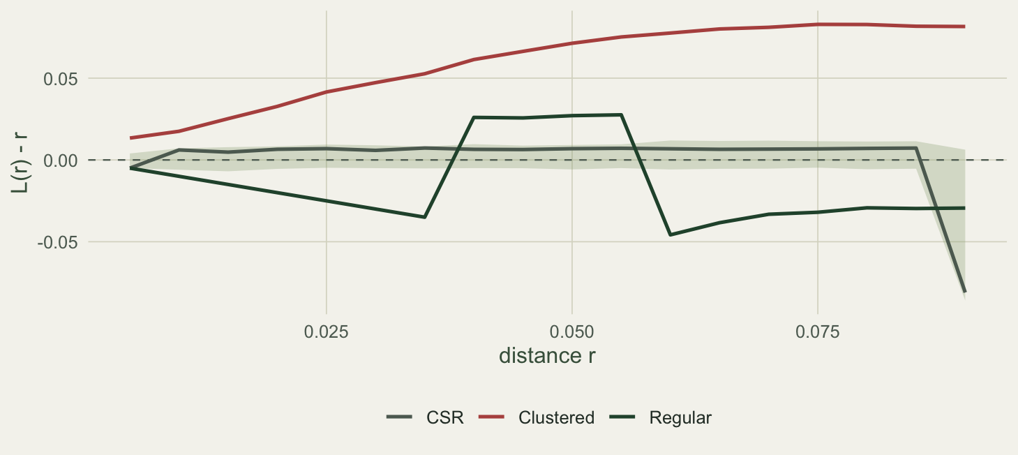

Figure 1: L(r) minus r for the three patterns, with the shaded pointwise envelope from 199 random simulations.

The regular pattern needs a careful reading, and it exposes something important about K. Its curve dips below the envelope at the shortest distances, the mark of the hard core that forbids close pairs. But it then rises back and even pokes above the envelope at intermediate distances before settling. That rebound is not a second, clustered scale hiding in the data. Because K is cumulative, the shortage of close pairs has to be made up somewhere: with a fixed number of points, a deficit at short range forces a surplus at longer range, and the surplus shows up as a bump. K remembers everything that happened at smaller distances and carries it forward.

The pair correlation function

The cure for that memory is to stop accumulating. The pair correlation function measures the density of pairs at exactly distance r, rather than within r, so each distance is judged on its own. It is estimated by smoothing the pairwise distances with a kernel and dividing out the geometry; under CSR it equals one at every distance. We use an Epanechnikov kernel with a small bandwidth.

g_fun <- function(pw, r_seq, h) {
  sapply(r_seq, function(r) {
    k <- (3 / (4 * h)) * (1 - ((r - pw$d) / h)^2)
    k[abs(r - pw$d) > h] <- 0
    (A / (n * (n - 1))) * 2 * sum(pw$w * k) / (2 * pi * r)
  })
}

h <- 0.012
obs_g <- lapply(patterns, function(p) g_fun(pair_dw(p$x, p$y), r_seq, h))

set.seed(7701)
g_sim <- matrix(NA, n_sim, length(r_seq))
for (s in 1:n_sim) g_sim[s, ] <- g_fun(pair_dw(runif(n), runif(n)), r_seq, h)
g_lo <- apply(g_sim, 2, min); g_hi <- apply(g_sim, 2, max)

data.frame(
  pattern  = names(obs_g),
  g_at_002 = sapply(obs_g, function(v) at(v, 0.02)),
  g_at_005 = sapply(obs_g, function(v) at(v, 0.05))
)

            pattern g_at_002 g_at_005
CSR             CSR 1.147151 1.051215
Clustered Clustered 6.592616 4.355852
Regular     Regular 0.000000 1.145564

g_df <- do.call(rbind, lapply(names(obs_g), function(nm)
  data.frame(pattern = nm, r = r_seq, val = obs_g[[nm]])))
g_df$pattern <- factor(g_df$pattern, levels = c("CSR", "Clustered", "Regular"))
genv_df <- data.frame(r = r_seq, lo = g_lo, hi = g_hi)

ggplot() +
  geom_ribbon(data = genv_df, aes(r, ymin = lo, ymax = hi), fill = te_sage, alpha = 0.30) +
  geom_hline(yintercept = 1, colour = te_faint, linetype = "dashed", linewidth = 0.4) +
  geom_line(data = g_df, aes(r, val, colour = pattern), linewidth = 0.9) +
  scale_colour_manual(values = c(CSR = te_faint, Clustered = te_rust, Regular = te_forest)) +
  labs(x = "distance r", y = "g(r)", colour = NULL) +
  theme_te() + theme(legend.position = "bottom")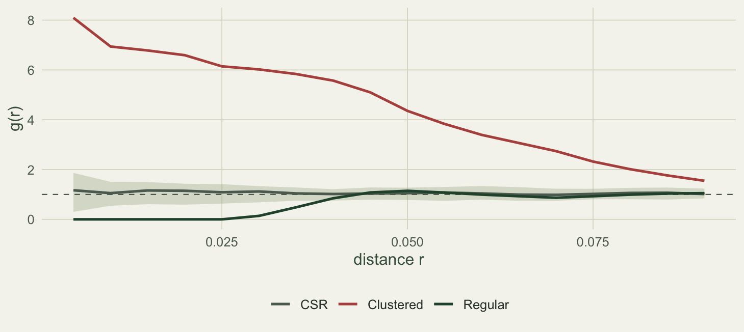

Figure 2: The pair correlation function for the three patterns, with the shaded envelope from 199 random simulations.

Read locally, the three patterns separate cleanly. The clustered pattern reaches a pair correlation above six at a distance of 0.02 and climbs past eight at the shortest distances: pairs are six to eight times denser than random there, decaying towards the envelope as the distance grows. The random pattern hovers near one. The regular pattern is exactly zero at a distance of 0.02, because no two points sit that close under the hard core, then climbs back into the envelope with none of the intermediate bump that troubled its K curve. For diagnosing the scale of interaction, the pair correlation function is usually the clearer of the two, precisely because it does not accumulate.

Choices that change the answer

Two settings deserve conscious choices rather than defaults. The first is the largest distance you interpret. Edge-corrected estimators grow noisier as r approaches the window size, because fewer point pairs and larger correction weights inflate the variance; a common rule keeps the sweep to a quarter of the shorter side or less, which is why the plots here stop at 0.09. The second is the envelope. A pointwise envelope from 199 simulations controls the error at each distance separately, but reading a whole curve against it tests many distances at once, so a curve can wander outside by chance at some scale even under randomness. Formal global tests exist that account for this, and for a confirmatory result they are worth the extra step; the pointwise envelope remains an excellent exploratory guide.

The bandwidth of the pair correlation function is a third choice, trading smoothness against resolution in the usual way. A narrow bandwidth resolves sharp features but is noisy; a wide one is smooth but blurs the scale of interaction.

When the intensity is not constant

Everything here assumes the pattern is stationary: the same expected density everywhere, so any structure in K reflects interaction between points rather than a trend in their abundance. Real maps rarely oblige. When density itself varies across the study area, a homogeneous K will report that variation as clustering, confounding a first-order trend with second-order interaction. The next post fits the trend explicitly and builds the inhomogeneous K that separates the two.

References

Ripley, B.D. (1977) Journal of the Royal Statistical Society Series B 39(2): 172-192. doi:10.1111/j.2517-6161.1977.tb01615.x

Besag, J.E. (1977) Journal of the Royal Statistical Society Series B 39(2): 193-195. doi:10.1111/j.2517-6161.1977.tb01616.x

Wiegand, T. and Moloney, K.A. (2014) Handbook of Spatial Point-Pattern Analysis in Ecology. Chapman and Hall/CRC. ISBN 978-1-4200-8254-8

Diggle, P.J. (2013) Statistical Analysis of Spatial and Spatio-Temporal Point Patterns, 3rd edition. Chapman and Hall/CRC. ISBN 978-1-4665-6023-9

Related tutorials

• Nearest-neighbour analysis and Clark-Evans in R
• Modelling inhomogeneous point patterns in R
• Complete spatial randomness and quadrat tests in R
• Spatial autocorrelation and Moran’s I in R