library(ggplot2)
library(dplyr)

ink <- "#16241d"; body <- "#2c3a31"; forest <- "#275139"; gold <- "#c9b458"
paper <- "#f5f4ee"; line_c <- "#dad9ca"; faint <- "#5d6b61"; sage <- "#93a87f"; red <- "#b5534e"

theme_te <- function(base = 12) {
  theme_minimal(base_size = base) +
    theme(panel.grid.minor = element_blank(),
          panel.grid.major = element_line(colour = line_c, linewidth = 0.3),
          plot.background = element_rect(fill = paper, colour = NA),
          panel.background = element_rect(fill = paper, colour = NA),
          axis.title = element_text(colour = body), axis.text = element_text(colour = faint),
          plot.title = element_text(colour = ink, face = "bold"),
          plot.subtitle = element_text(colour = faint),
          legend.title = element_text(colour = body), legend.text = element_text(colour = faint))
}Removal and depletion sampling in R
R
abundance
detection
ecology tutorial
Estimate closed-population size from a declining series of removal catches. Fit the Zippin removal model and the Leslie-DeLury depletion regression in R.
Suppose you sample a closed patch several times and remove every individual you catch: electrofishing a stream reach, trapping small mammals for a translocation, hand-collecting amphibians from a pond. Each pass catches fewer than the last, because the pool of animals left to catch is shrinking. That decline carries information. If catches drop steeply, few animals remain and the population was small; if they drop gently, many remain and the population was large.
Removal sampling turns that intuition into an estimate. The total caught is only a lower bound, since some animals are never taken, but the rate of decline lets you estimate both the per-pass catch probability and the starting population size. This post fits the classical removal model of Moran (1951) and Zippin (1958) by hand with optim, recovers the same population size from the Leslie-DeLury depletion regression, and shows why two passes are rarely enough.
The model
Work in a closed patch with k removal passes. Before pass j there are some animals left, and each is caught and removed with probability p. If the starting population is N and S_{j-1} animals have already been removed, the catch on pass j is binomial:
\[x_j \sim \text{Binomial}\!\left(N - S_{j-1},\; p\right).\]
Because animals are removed rather than replaced, the expected catch shrinks geometrically: the first pass takes about pN, the next about p of what remains, and so on. The likelihood is the product of these binomial terms, with two unknowns, N and p. The steepness of the decline identifies p, and p together with the first catch pins down N.
Simulating a depletion survey
We take a patch of 220 animals, five passes, and a catch probability of 0.40. Setting the seed just before the draws keeps the sequence reproducible.
set.seed(17)
Ntrue <- 220; p_true <- 0.40; k <- 5

catch <- integer(k)
remaining <- Ntrue
for (j in 1:k) {
  cj <- rbinom(1, remaining, p_true)   # each remaining animal caught with prob p
  catch[j] <- cj
  remaining <- remaining - cj          # removed, not returned
}
catch
[1] 79 58 36 21 8Tc <- sum(catch) # total caught
cum_before <- c(0, cumsum(catch)[-k]) # animals already removed before each pass
c(total_caught = Tc, true_N = Ntrue, never_caught = Ntrue - Tc)total_caught true_N never_caught
202 220 18 The five passes take 79, 58, 36, 21 and 8 animals. The total caught, 202, is a firm lower bound on the population: at least that many were there. It misses the 18 animals, about 8%, that survived all five passes uncaught. The task is to estimate those from the shape of the decline.
Fitting the model by hand
The negative log-likelihood sums the binomial terms. To keep N above the total catch and p inside the unit interval, we optimise on transformed scales and read the estimates back afterwards.
nll <- function(par) {
  N <- Tc + exp(par[1])          # N is at least the total already caught
  p <- plogis(par[2])
  remain <- N - cum_before
  if (any(remain < catch)) return(1e6)
  -sum(lchoose(remain, catch) + catch * log(p) + (remain - catch) * log(1 - p))
}

o <- optim(c(log(20), qlogis(0.35)), nll, method = "BFGS", hessian = TRUE)
N_hat <- Tc + exp(o$par[1])
p_hat <- plogis(o$par[2])

V <- solve(o$hessian)
se_N <- sqrt(V[1, 1]) * (N_hat - Tc)          # delta method for N = Tc + exp(.)
se_p <- sqrt(V[2, 2]) * p_hat * (1 - p_hat)   # delta method for p
round(c(N_hat = N_hat, se_N = se_N, p_hat = p_hat, se_p = se_p), 3)
N_hat se_N p_hat se_p
220.035 7.368 0.391 0.035 The estimate of the population is 220 individuals with a standard error of about 7, so a Wald interval of roughly 206 to 235, and the catch probability comes out at 0.39 against the true 0.40. The model has recovered the 18 uncaught animals from nothing but the rate at which catches fell.
The depletion regression
There is an older graphical route that is worth knowing, because it makes the logic visible. The expected catch on a pass is p times the number remaining, which is p(N - S_{j-1}). Plotting the catch against the cumulative number already removed should give a straight line: its slope is minus the catch probability, and the point where it crosses zero is the population size, the number at which nothing is left to catch. This is the Leslie-DeLury method (Leslie and Davis; DeLury 1947).
exp_catch <- p_hat * (N_hat - cum_before)
d1 <- data.frame(pass = factor(1:k), catch = catch, fit = exp_catch)

ggplot(d1, aes(pass, catch)) +
  geom_col(width = 0.6, fill = forest) +
  geom_line(aes(x = as.numeric(pass), y = fit), colour = red, linewidth = 0.8) +
  geom_point(aes(x = as.numeric(pass), y = fit), colour = red, size = 2.4) +
  labs(title = "Catches decline as animals are removed",
       subtitle = "Observed catch per pass (bars) and the fitted removal model (line)",
       x = "Removal pass", y = "Individuals caught") +
  theme_te()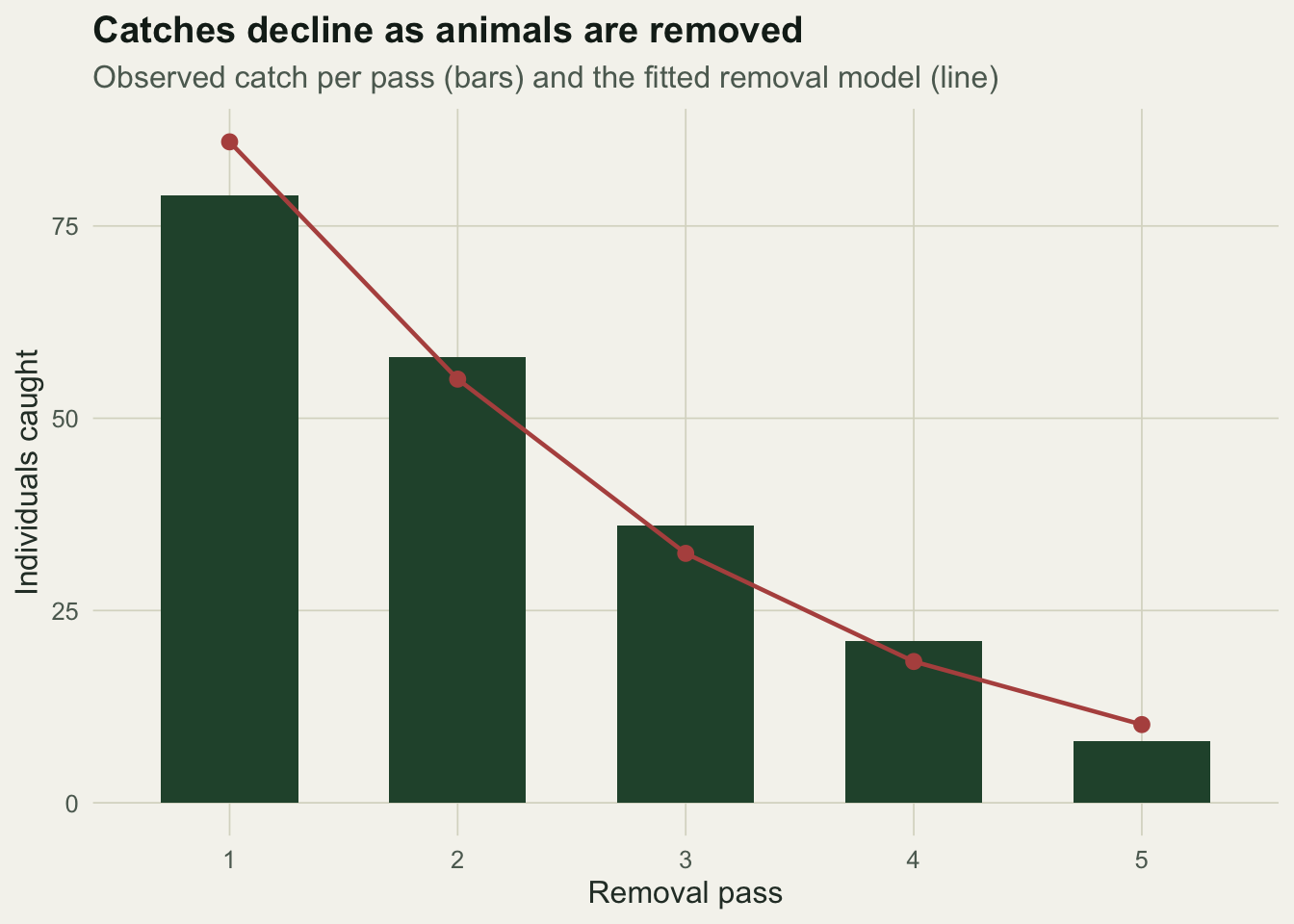
les <- lm(catch ~ cum_before)
sl <- coef(les)[2]; ic <- coef(les)[1]
N_les <- -ic / sl                 # cumulative catch at which the line hits zero
p_les <- -sl                      # slope is minus the catch probability
c(N_leslie = N_les, p_leslie = p_les, r2 = summary(les)$r.squared)
N_leslie.(Intercept) p_leslie.cum_before r2
228.8322604 0.3599678 0.9821357 ggplot(d1, aes(cum_before, catch)) +
geom_abline(slope = sl, intercept = ic, colour = forest, linewidth = 0.7) +
geom_point(colour = ink, size = 2.6) +
geom_hline(yintercept = 0, colour = faint, linewidth = 0.3) +
geom_point(aes(x = N_les, y = 0), colour = red, size = 3) +
annotate("text", x = N_les, y = 6, label = sprintf("N = %.0f", N_les),
colour = red, hjust = 1.05, size = 3.6) +
labs(title = "Depletion regression estimates population size",
subtitle = "Catch per pass falls linearly with the number already removed",
x = "Cumulative catch before the pass", y = "Catch on the pass (CPUE)") +
theme_te()Warning in geom_point(aes(x = N_les, y = 0), colour = red, size = 3): All aesthetics have length 1, but the data has 5 rows.
ℹ Please consider using `annotate()` or provide this layer with data containing
a single row.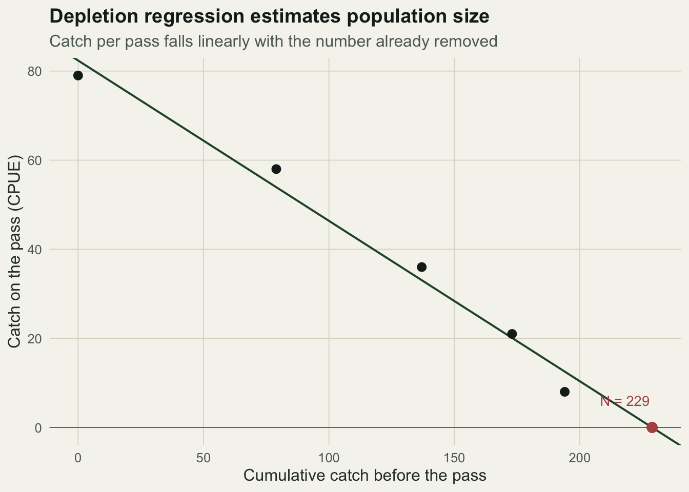
The regression is nearly linear here, with an R-squared of 0.98, and its x-intercept lands at 229 with an implied catch probability of 0.36. That is close to the likelihood estimate of 220, and the small gap is the usual difference between a least-squares fit to the catches and the exact binomial likelihood. The regression is quick and transparent, but the likelihood is preferable for inference because it gives proper confidence intervals rather than a regression slope on non-independent points.
An interval for the population
The confidence interval for a population size is often asymmetric, because the data rule out small populations more sharply than large ones. The profile likelihood shows this directly: fix a candidate N, take the best p for it, and record the log-likelihood. The values of N within a set drop from the peak form the interval.
Ngrid <- Tc:(Tc + 250)
profll <- sapply(Ngrid, function(Nn) {
  remain <- Nn - cum_before
  ph <- Tc / sum(remain)          # closed-form best p for this N
  if (ph <= 0 || ph >= 1) return(-Inf)
  sum(dbinom(catch, remain, ph, log = TRUE))
})
Nhat_int <- Ngrid[which.max(profll)]
cut <- max(profll) - qchisq(0.95, 1) / 2
Nci_lr <- range(Ngrid[profll >= cut])
c(N_hat = Nhat_int, lo = Nci_lr[1], hi = Nci_lr[2])
N_hat lo hi
220 209 239 d3 <- data.frame(N = Ngrid, rll = profll - max(profll))
d3 <- d3[d3$rll > -6, ]
ggplot(d3, aes(N, rll)) +
annotate("rect", xmin = Nci_lr[1], xmax = Nci_lr[2], ymin = -Inf, ymax = Inf,
alpha = 0.08, fill = gold) +
geom_line(colour = forest, linewidth = 0.7) +
geom_hline(yintercept = -qchisq(0.95, 1) / 2, linetype = "dashed", colour = faint) +
geom_vline(xintercept = Nhat_int, colour = red, linewidth = 0.5) +
labs(title = "Profile likelihood gives the interval for N",
subtitle = "Relative log-likelihood; dashed line is the 95% cut, shaded band the interval",
x = "Population size N", y = "Relative log-likelihood") +
theme_te()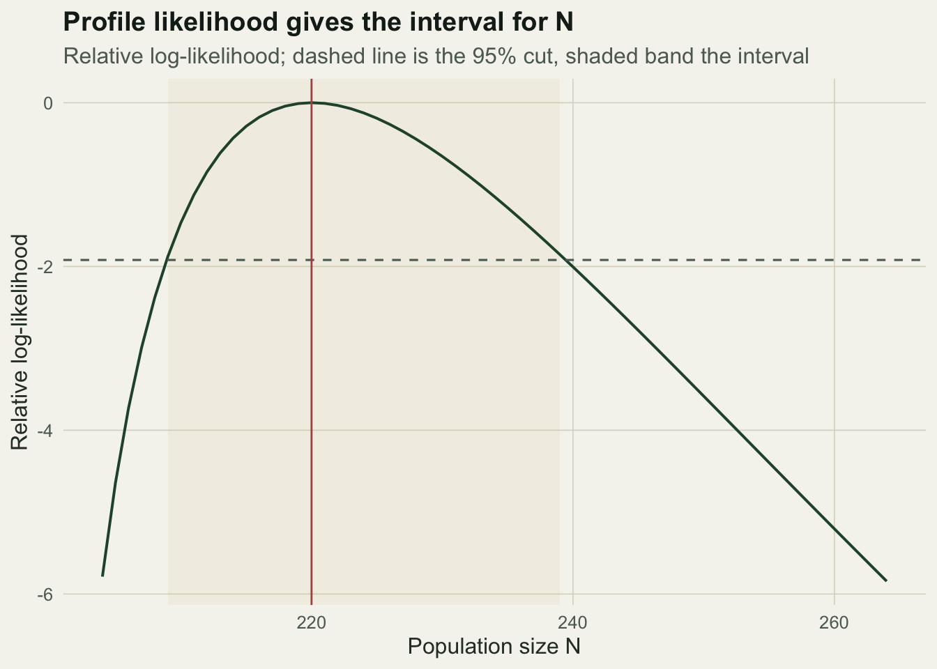
The likelihood-ratio interval runs from 209 to 239, wider above the estimate than below, which the symmetric Wald interval from the Hessian cannot show. Reporting the profile interval is the more honest choice for a bounded quantity like a count.
Why two passes are rarely enough
It is tempting to run just two passes and use the classic two-sample formula. On this data that gives a very different answer.
N2 <- catch[1]^2 / (catch[1] - catch[2])
p2 <- (catch[1] - catch[2]) / catch[1]
c(N_two_pass = N2, p_two_pass = p2)
N_two_pass p_two_pass
297.1904762 0.2658228 Two passes here return a population of 297, far above the full-data estimate of 220, because the drop from the first catch to the second happened to be gentle and two points cannot tell a gentle real decline from sampling noise. Three or more passes let the later catches correct that first impression. The practical guidance is to run enough passes that the last catch is a small fraction of the first, so the decline is clearly resolved.
Assumptions and when it fails
The removal model rests on closure and constant catchability. Nothing may enter or leave the patch during sampling, and every animal must have the same catch probability on every pass. Both are easy to break. If handling makes animals trap-shy, catchability falls over passes, the decline steepens artificially, and the model underestimates the population. If animals differ in catchability, the easy ones go first and the apparent decline again overstates depletion. Carle and Strub (1978) give a weighted estimator that eases the equal-catchability assumption, and Seber and Le Cren treat catches that are large relative to the population. Where individuals can be marked and released instead of removed, a capture-recapture design avoids depleting the population at all.
References
Moran 1951 Biometrika 38(3-4):307-311 (10.1093/biomet/38.3-4.307)
Zippin 1958 Journal of Wildlife Management 22(1):82-90 (10.2307/3797301)
DeLury 1947 Biometrics 3(4):145-167 (10.2307/3001390)
Carle and Strub 1978 Biometrics 34(4):621-630 (10.2307/2530381)