kfs_irw <- function(times, y, sig2, tau2){
  n <- length(times)
  Amk <- function(dt) matrix(c(1,0,dt,1),2,2)
  Qmk <- function(dt) sig2*matrix(c(dt^3/3, dt^2/2, dt^2/2, dt),2,2)
  Z <- matrix(c(1,0),1,2)
  a <- c(if(!is.na(y[1])) y[1] else 0, 0)
  P <- matrix(c(1e6,0,0,1e2),2,2)                # vague prior
  ll <- 0
  af<-matrix(NA,n,2); Pf<-vector("list",n); ap<-matrix(NA,n,2); Pp<-vector("list",n); Al<-vector("list",n)
  for(t in 1:n){
    if(t==1){ A<-diag(2); Q<-matrix(0,2,2) } else { dt<-times[t]-times[t-1]; A<-Amk(dt); Q<-Qmk(dt) }
    ap_t<-as.vector(A%*%a); Pp_t<-A%*%P%*%t(A)+Q
    Al[[t]]<-A; ap[t,]<-ap_t; Pp[[t]]<-Pp_t
    if(!is.na(y[t])){
      v<-y[t]-as.vector(Z%*%ap_t); Ft<-as.vector(Z%*%Pp_t%*%t(Z))+tau2
      K<-as.vector(Pp_t%*%t(Z))/Ft
      a<-ap_t+K*v; P<-Pp_t-(K%*%Z)%*%Pp_t
      if(t>1) ll<-ll-0.5*(log(2*pi)+log(Ft)+v^2/Ft)
    } else { a<-ap_t; P<-Pp_t }                   # gap: predict only
    af[t,]<-a; Pf[[t]]<-P
  }
  as<-af; Ps<-Pf                                  # RTS smoother
  for(t in (n-1):1){
    A1<-Al[[t+1]]; Pp1<-Pp[[t+1]]; C<-Pf[[t]]%*%t(A1)%*%solve(Pp1)
    as[t,]<-af[t,]+as.vector(C%*%(as[t+1,]-ap[t+1,]))
    Ps[[t]]<-Pf[[t]]+C%*%(Ps[[t+1]]-Pp1)%*%t(C)
  }
  list(ll=ll, sm_p=as[,1], sm_psd=sapply(Ps, function(M) sqrt(max(M[1,1],0))))
}Regularising irregular animal tracks
movement ecology
state-space models
Kalman filter
R
ecology tutorial
Turn irregular, gappy animal tracks into a regular series with a continuous-time integrated random walk and Kalman smoother in base R, with honest uncertainty over gaps.
Most movement methods assume fixes arrive at even intervals. Real tags rarely oblige: an Argos device reports when a satellite passes, a GPS tag drops fixes under canopy, and a battery-saving duty cycle leaves long stretches blank. Interpolating linearly onto a regular grid is the usual quick fix, but a straight line between two noisy points ignores both the location error and the way the animal actually moves, and it invents certainty it does not have. A continuous-time state-space model does the job properly: it works in real time rather than in fix number, denoises as it goes, and reports how uncertain each reconstructed position is.
A movement model that runs in continuous time
The discrete correlated random walk of the previous post needs even steps. Its continuous-time analogue is the integrated random walk: velocity follows a random walk in continuous time, and position is its integral. Over a gap of length \(\Delta t\) the state (position, velocity) evolves through
\[A(\Delta t) = \begin{pmatrix} 1 & \Delta t \\ 0 & 1 \end{pmatrix}, \qquad Q(\Delta t) = \sigma^2 \begin{pmatrix} \Delta t^3/3 & \Delta t^2/2 \\ \Delta t^2/2 & \Delta t \end{pmatrix}.\]
The process noise grows with the gap: the longer the tag is silent, the more the animal could have wandered, and \(Q\) encodes exactly that. This is the model behind widely used tools for Argos data, here written from scratch. Because the transition depends only on \(\Delta t\), the same Kalman filter handles any spacing, and a missing observation simply skips the update step.
An irregular track with a reporting gap
We simulate a true track on a fine grid, then keep an uneven, thinned set of fixes, deliberately dropping all fixes in one window so the tag falls silent for a stretch, as a real device does when it loses contact.
set.seed(8143)
sig_t <- 1.0; tau_t <- 4.0
dt0 <- 0.25; Tmax <- 100; fg <- seq(0, Tmax, by=dt0); nf <- length(fg)
simcoord <- function(){
  p<-numeric(nf); v<-numeric(nf); p[1]<-0; v[1]<-rnorm(1,0,1)
  for(i in 2:nf){
    Q<-sig_t^2*matrix(c(dt0^3/3,dt0^2/2,dt0^2/2,dt0),2,2)
    e<-MASS::mvrnorm(1,c(0,0),Q); v[i]<-v[i-1]+e[2]; p[i]<-p[i-1]+dt0*v[i-1]+e[1]
  }
  p
}
px<-simcoord(); py<-simcoord()

set.seed(8144)
elig <- which(fg > 0 & fg < Tmax & !(fg >= 44 & fg <= 58))   # silent window
keep <- sort(sample(elig, 56)); keep <- c(1, keep, nf)
ot <- fg[keep]
ox <- px[keep] + rnorm(length(keep),0,tau_t)
oy <- py[keep] + rnorm(length(keep),0,tau_t)
n_obs <- length(ot); gap_med <- median(diff(ot)); gap_max <- max(diff(ot))
c(n_obs=n_obs, median_gap=round(gap_med,2), max_gap=round(gap_max,2))
n_obs median_gap max_gap
58.00 1.25 14.75 The 58 fixes have a median spacing of 1.25 time units but a longest gap of 14.75, the deliberate silent window.
Fitting and reconstructing
We estimate the process and observation standard deviations by maximum likelihood, then predict the state at a regular grid by treating the grid times as extra, unobserved time points. The smoother returns both a position and its standard deviation at every grid point.
nll <- function(par){ s2<-exp(par[1]); h2<-exp(par[2])
  -(kfs_irw(ot,ox,s2,h2)$ll + kfs_irw(ot,oy,s2,h2)$ll) }
fit <- optim(c(log(1),log(16)), nll, method="Nelder-Mead", control=list(reltol=1e-10,maxit=3000))
sig_h<-sqrt(exp(fit$par[1])); tau_h<-sqrt(exp(fit$par[2]))
c(sigma=round(sig_h,3), tau=round(tau_h,3))
sigma tau
1.020 3.926 grid <- seq(0, Tmax, by=1.0)
utimes <- sort(unique(c(ot, grid)))
yx <- rep(NA_real_, length(utimes)); yx[match(ot, utimes)] <- ox
yy <- rep(NA_real_, length(utimes)); yy[match(ot, utimes)] <- oy
smx <- kfs_irw(utimes, yx, sig_h^2, tau_h^2)
smy <- kfs_irw(utimes, yy, sig_h^2, tau_h^2)
gi <- match(grid, utimes)
gx<-smx$sm_p[gi]; gy<-smy$sm_p[gi]; gsd<-smx$sm_psd[gi]
nx <- approx(ot, ox, xout=grid)$y; ny <- approx(ot, oy, xout=grid)$y # naive interpolation
tx <- px[match(grid, fg)]; ty <- py[match(grid, fg)]
rmse<-function(ex,ey) sqrt(mean((ex-tx)^2+(ey-ty)^2))
rmse_naive<-rmse(nx,ny); rmse_sm<-rmse(gx,gy)
c(rmse_naive=round(rmse_naive,2), rmse_smoother=round(rmse_sm,2),
sd_min=round(min(gsd),2), sd_max=round(max(gsd),2)) rmse_naive rmse_smoother sd_min sd_max
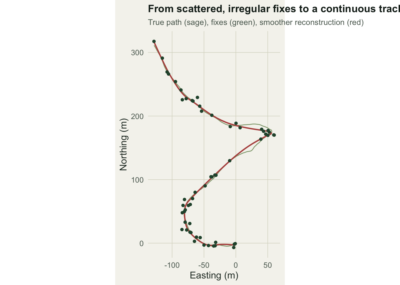
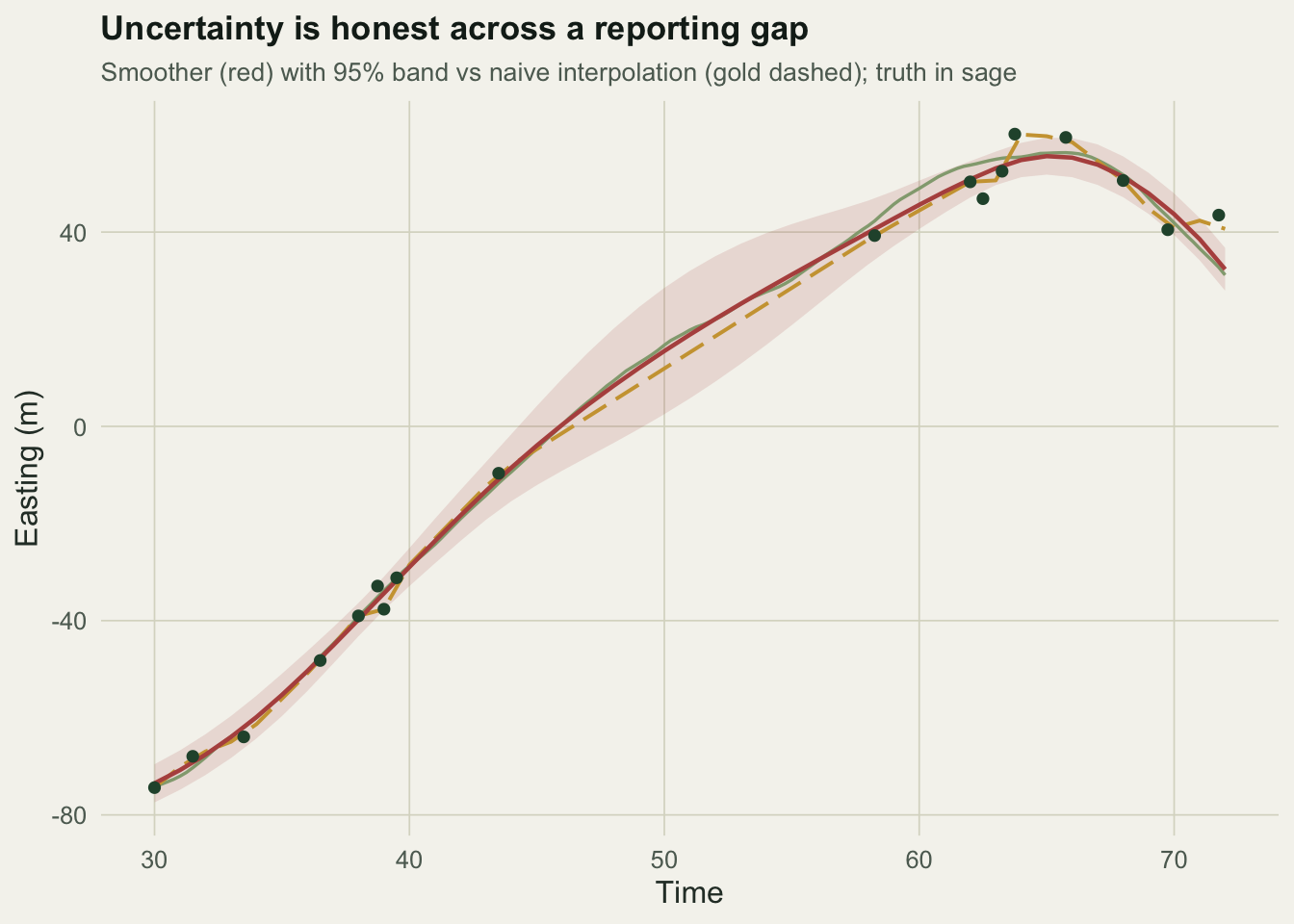
4.75 3.54 1.56 6.70 Estimation recovers the truth well: process standard deviation 1.02 against a true 1, and observation standard deviation 3.926 against 4. On the regular grid the smoother sits 3.54 units from the true path on average, against 4.75 for naive linear interpolation. The more telling number is the uncertainty: the smoother’s standard deviation ranges from 1.56 next to a fix up to 6.7 in the middle of the silent window. The band balloons exactly where the data are absent, which is the honest thing to report.
Can we trust the two variances?
Separating movement from observation error rests on the model seeing enough closely spaced fixes to tell a genuine wiggle from noise. To show when that breaks, profile the likelihood over the observation standard deviation, re-optimising the process term at each value, for the full data and for a thinned subset with larger gaps.
taus <- seq(2.0, 6.5, by=0.25)
prof <- function(t_ot,t_ox,t_oy) sapply(taus, function(tt){
  f<-optimise(function(ls){ s2<-exp(ls)
    -(kfs_irw(t_ot,t_ox,s2,tt^2)$ll + kfs_irw(t_ot,t_oy,s2,tt^2)$ll) }, c(log(1e-3),log(30)))
  -f$objective })
pll <- prof(ot,ox,oy)
set.seed(8145)
thin <- sort(c(1, sample(2:(n_obs-1), 20), n_obs))
pll2 <- prof(ot[thin], ox[thin], oy[thin])
w_full <- range(taus[pll  >= max(pll)-2])
w_thin <- range(taus[pll2 >= max(pll2)-2])
rbind(full=round(w_full,2), thinned=round(w_thin,2))
[,1] [,2]
full 3.50 4.50
thinned 2.75 4.75With the full 58 fixes the profile confidence interval for the observation standard deviation runs from 3.5 to 4.5, a tight window around the true value of 4. Thin the track to 22 fixes and the interval widens to 2.75 through 4.75. The two variances are separable when fixes are dense enough to reveal the process between the noise, and confounded when they are not. This is the identifiability limit that recurs across state-space movement models: dense data make the split clean, sparse or very noisy data make it fragile.
References
Rauch, Tung and Striebel 1965. AIAA Journal 3(8):1445-1450 (10.2514/3.3166)
Johnson, London, Lea and Durban 2008. Ecology 89(5):1208-1215 (10.1890/07-1032.1)
Jonsen, Flemming and Myers 2005. Ecology 86(11):2874-2880 (10.1890/04-1852)
Auger-Methe, Field, Albertsen, Derocher, Lewis, Jonsen and Mills Flemming 2016. Scientific Reports 6:26677 (10.1038/srep26677)
Knape 2008. Ecology 89(11):2994-3000 (10.1890/08-0071.1)
Durbin and Koopman 2012. Time Series Analysis by State Space Methods, 2nd edn. ISBN 978-0-19-964117-8