library(ggplot2)
library(patchwork)
library(quantreg)

te_paper  <- "#f5f4ee"
te_ink    <- "#16241d"
te_body   <- "#2c3a31"
te_forest <- "#275139"
te_rust   <- "#b5534e"
te_gold   <- "#c9b458"
te_line   <- "#dad9ca"

theme_datasheet <- function() {
  theme_minimal(base_size = 12) +
    theme(plot.background  = element_rect(fill = te_paper, colour = NA),
          panel.background = element_rect(fill = te_paper, colour = NA),
          panel.grid.major = element_line(colour = te_line, linewidth = 0.3),
          panel.grid.minor = element_blank(),
          text             = element_text(colour = te_body),
          plot.title       = element_text(colour = te_ink, face = "bold"),
          plot.subtitle    = element_text(colour = te_body),
          axis.text        = element_text(colour = te_body))
}Confidence intervals in quantile regression
R
quantile regression
confidence intervals
quantreg
simulation
ecology tutorial
The default quantreg interval is a 90 per cent rank interval that assumes equal spread. Measuring in R how it undercovers when the scatter fans out with x.
Sixty sapling plots along a gradient of canopy openness, one height increment per plot, and the question is not how fast the average sapling grows in more light but how fast the best ones can. That is an upper quantile, and the ninetieth percentile slope is what the study is for. In the open plots a few saplings shoot up and many are held back by browsing, drought or competition, so the scatter fans out as light increases. The fan is the reason for fitting a quantile regression in the first place: Cade and Noon 2003 introduce the method to ecologists with exactly this picture of unequal spread under a limiting factor.
This site already has the fit. Quantile regression in ecology builds the check loss by hand with optim and checks the result against the standard linear programming fit; no interval appears in it. Heteroscedasticity and limiting factors and Checking a quantile regression put intervals on quantile slopes with a case bootstrap that resamples plots, and the second of them warns that a tail slope resting on three points cannot be trusted whatever width the bootstrap returns. Neither measures how often any of those intervals contains the true slope. The pairs bootstrap measured below resamples plots in the same way, although its interval here is built from the bootstrap standard error rather than from percentiles.
Most people who fit a quantile regression in R do not write the bootstrap. They call rq() from quantreg and then summary(), and they read the two columns headed lower bd and upper bd. This post measures what those two columns are and how often they cover. The answer is documented in ?summary.rq and ?rq.fit.br: below 1001 observations the default is a rank inversion interval (Koenker 1994) at ninety per cent, computed under the assumption that the errors are independent and identically distributed. Ninety rather than ninety five is a stated argument, not a defect. The equal spread assumption is the part that matters for ecology, because the data that motivated the quantile regression break it.
What summary() prints for sixty plots
The simulated plots have canopy openness spread evenly from zero to ten, in tens of per cent. The height increment is a baseline of ten centimetres, a mean rise of 0.3 centimetres per ten points of openness, and a right skewed error: a gamma variate with shape two, centred on its mean and scaled by a spread that is 2.5 + g * (x - 5). With g = 0 the spread is the same everywhere; with g = 0.4 it grows from 0.5 in the shaded plots to 4.5 in the open ones, which is the fan.
qr_version <- as.character(packageVersion("quantreg"))
g_fan  <- 0.4        # spread 0.5 at x = 0, 4.5 at x = 10
g_flat <- 0          # spread 2.5 everywhere
gam_shape <- 2       # gamma error, mean 2, centred before scaling

sim_plots <- function(n, g) {
  open <- runif(n, 0, 10)
  spread <- 2.5 + g * (open - 5)
  data.frame(open = open,
             growth = 10 + 0.3 * open + spread * (rgamma(n, gam_shape, 1) - gam_shape))
}
# the tau quantile of growth given open is linear in open, with this slope
q_slope <- function(tau, g) 0.3 + g * (qgamma(tau, gam_shape, 1) - gam_shape)

set.seed(3450)
plots <- sim_plots(60, g_fan)
tau_up <- 0.9
b_true <- q_slope(tau_up, g_fan)
fit <- rq(growth ~ open, tau = tau_up, data = plots)
Because the error is a fixed distribution stretched by a spread that is linear in openness, every conditional quantile is a straight line, and its slope is the mean slope plus g times the centred gamma quantile. For the ninetieth percentile in the fan that is 1.056 centimetres per ten points of openness, against 0.3 for the mean. With g = 0 every quantile slope equals 0.3.
warn_msg <- character(0)
s_def <- withCallingHandlers(summary(fit), warning = function(w) {
  warn_msg <<- c(warn_msg, conditionMessage(w)); invokeRestart("muffleWarning")
})
s_def
Call: rq(formula = growth ~ open, tau = tau_up, data = plots)

tau: [1] 0.9

Coefficients:
            coefficients lower bd upper bd
(Intercept) 10.05600      8.54960 12.86826
open         1.39943      0.77036  1.81479
summary_rq <- getS3method("summary", "rq")
stopifnot(is.null(formals(summary_rq)$se),
isFALSE(formals(summary_rq)$covariance),
formals(rq.fit.br)$alpha == 0.1,
isTRUE(formals(rq.fit.br)$iid),
any(grepl("n < 1001", deparse(summary_rq), fixed = TRUE)))
# the printed table is rq.fit.br(ci = TRUE) with its defaults
x_mat <- cbind(1, plots$open)
br_def <- suppressWarnings(rq.fit.br(x_mat, plots$growth, tau = tau_up, ci = TRUE))
stopifnot(isTRUE(all.equal(unname(s_def$coefficients), unname(br_def$coefficients))))
# the switch: 1000 rows still get the rank interval, 1001 rows get nid
set.seed(3449)
big <- sim_plots(1001, g_fan)
cols_1000 <- colnames(suppressWarnings(summary(rq(growth ~ open, tau = tau_up,
data = big[1:1000, ])))$coefficients)
cols_1001 <- colnames(suppressWarnings(summary(rq(growth ~ open, tau = tau_up,
data = big)))$coefficients)
stopifnot(identical(cols_1000, c("coefficients", "lower bd", "upper bd")),
identical(cols_1001, c("Value", "Std. Error", "t value", "Pr(>|t|)")))
# the warning comes from the interval step, and only because 60 * 0.9 is whole
warn_fit <- tryCatch({ rq(growth ~ open, tau = tau_up, data = plots); "none" },
warning = function(w) conditionMessage(w))
warn_59 <- tryCatch({ rq.fit.br(x_mat[-60, ], plots$growth[-60], tau = tau_up,
ci = TRUE); "none" },
warning = function(w) conditionMessage(w))
stopifnot(identical(warn_msg, "Solution may be nonunique"),
identical(warn_fit, "none"), identical(warn_59, "none"))
def_lo <- s_def$coefficients[2, 2]; def_hi <- s_def$coefficients[2, 3]
# the interval step warns whenever n * tau is whole: 200 datasets at 59, 60, 61 plots
set.seed(3453)
nonuniq <- vapply(c(59, 60, 61), function(n) sum(replicate(200, { d <- sim_plots(n, g_fan)
tryCatch({ rq.fit.br(cbind(1, d$open), d$growth, tau = tau_up, ci = TRUE); "none" },
warning = function(w) conditionMessage(w)) == "Solution may be nonunique" })), 0)
stopifnot(identical(nonuniq, c(0, 200, 0)))
# nid and the xy bootstrap report a t test on n - 2 degrees of freedom
s_nid_chk <- suppressWarnings(summary(fit, se = "nid"))$coefficients
set.seed(3454)
s_boot_chk <- summary(fit, se = "boot", bsmethod = "xy", R = 50)$coefficients
stopifnot(isTRUE(all.equal(s_nid_chk[2, 4],
2 * (1 - pt(abs(s_nid_chk[2, 3]), nrow(plots) - 2)))),
isTRUE(all.equal(s_boot_chk[2, 4],
2 * (1 - pt(abs(s_boot_chk[2, 3]), nrow(plots) - 2)))))The slope row reads 1.399 with bounds 0.770 and 1.815. The chunk above checks that table against the installed quantreg 6.1, so that a change of version would stop the knit instead of changing the meaning of this paragraph silently. The se argument of summary.rq defaults to NULL, and the source then picks "rank" when there are fewer than 1001 rows and no covariance matrix is requested, otherwise "nid": a model on 1000 rows prints the columns “coefficients”, “lower bd”, “upper bd”, and on 1001 rows “Value”, “Std. Error”, “t value”, “Pr(>|t|)”. The rank interval is computed by rq.fit.br() with its own defaults, alpha = 0.1 and iid = TRUE, and the printed numbers are identical to a direct call of that function. The same lines are in the quantreg 6.1 source in the CRAN mirror on GitHub, read on 27 September 2026.
The interval is also asymmetric around the estimate, which a standard error cannot be, and there is no p value in the table. That is the rank inversion at work: the bounds are the slopes at which a rank score test, in the form given by Koenker 1994, stops rejecting at the ten per cent level.
The summary() call also raised the warning “Solution may be nonunique”, which the chunk captured rather than printed. It is issued by the interval step, not by the fit: rq() alone is silent on the same data, and the chunk checks that too. Sixty times 0.9 is a whole number. The rank test behind the interval holds the slope at a trial value and fits only the intercept, and with a whole number of points to go below that line the check loss is flat across a small range of intercepts, in the same way that any value between the middle two is a median of an even number of values. Drop one plot and the warning does not appear. Over 200 fresh datasets at each size, the interval step warned for all 200 with 60 plots and for none with 59 or 61. It says nothing about the coverage of the interval.
set.seed(3448)
show_n <- 250
show <- rbind(cbind(sim_plots(show_n, g_flat), spread = "equal spread (g = 0)"),
              cbind(sim_plots(show_n, g_fan), spread = "fan (g = 0.4)"))
show$spread <- factor(show$spread, levels = c("equal spread (g = 0)", "fan (g = 0.4)"))
lines_df <- do.call(rbind, lapply(levels(show$spread), function(s) {
  g_s <- if (grepl("fan", s)) g_fan else g_flat
  d_s <- show[show$spread == s, ]
  cf <- coef(rq(growth ~ open, tau = tau_up, data = d_s))
  q_int <- 10 + (2.5 - 5 * g_s) * (qgamma(tau_up, gam_shape, 1) - gam_shape)
  data.frame(spread = s, line = c("true 0.9 quantile", "fitted 0.9 quantile"),
             a = c(q_int, cf[1]), b = c(q_slope(tau_up, g_s), cf[2]))
}))
lines_df$spread <- factor(lines_df$spread, levels = levels(show$spread))
ggplot(show, aes(open, growth)) +
  geom_point(colour = te_forest, alpha = 0.45, size = 1.4) +
  geom_abline(data = lines_df, aes(intercept = a, slope = b, colour = line,
                                   linetype = line), linewidth = 0.9) +
  facet_wrap(~ spread) +
  scale_colour_manual(values = c(te_rust, te_ink), name = NULL) +
  scale_linetype_manual(values = c("solid", "dashed"), name = NULL) +
  labs(x = "canopy openness (tens of per cent)", y = "height increment (cm)",
       title = "The same mean trend, two kinds of scatter",
       subtitle = "n = 250 per panel, tau = 0.9") +
  theme_datasheet() + theme(legend.position = "bottom")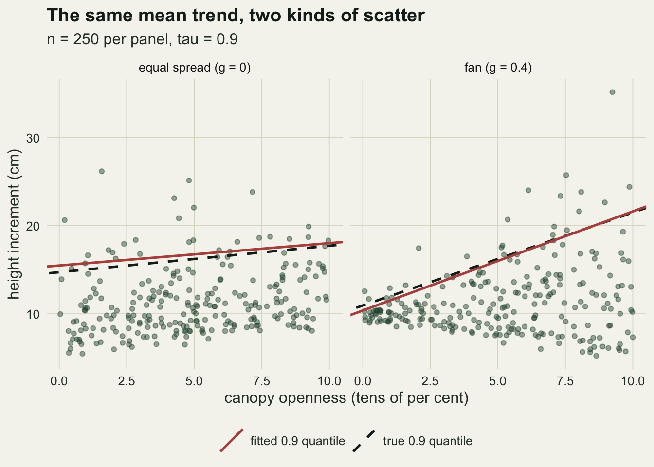
How often each interval covers
Five intervals for the slope, computed on the same simulated datasets. The default is the ninety per cent rank interval under equal spread. The second is the same rank interval at alpha = 0.05, which is what a reader who wants ninety five per cent would type first. The third is the rank interval at ninety five per cent with iid = FALSE, the variant of Koenker and Machado 1999 that the help page offers for errors that are not identically distributed. The fourth is se = "nid", a sandwich standard error with a local estimate of the sparsity (Hendricks and Koenker 1992), and the fifth is se = "boot" with bsmethod = "xy", the pairs bootstrap, with 200 resamples. Both standard error methods give an interval as the estimate plus or minus a t quantile on n minus 2 degrees of freedom, the same reference distribution summary() uses for their p values.
The design has two quantile levels, two sample sizes and the two generators, and three further levels of g at the larger sample size and the upper quantile. All of it was fixed before any coverage was computed.
n_rep  <- 1000       # datasets per cell, fixed in advance
r_boot <- 200        # pairs bootstrap resamples
arms <- c("default: rank 90%, iid", "rank 95%, iid", "rank 95%, iid = FALSE",
          "nid 95%", "xy bootstrap 95%")
nominal <- c(0.90, 0.95, 0.95, 0.95, 0.95)

one_rep <- function(d, tau, b_true) {
  x_mat <- cbind(1, d$open); t_crit <- qt(0.975, nrow(d) - 2)
  r90  <- suppressWarnings(rq.fit.br(x_mat, d$growth, tau = tau, ci = TRUE))
  r95  <- suppressWarnings(rq.fit.br(x_mat, d$growth, tau = tau, ci = TRUE,
                                     alpha = 0.05))
  r95n <- suppressWarnings(rq.fit.br(x_mat, d$growth, tau = tau, ci = TRUE,
                                     alpha = 0.05, iid = FALSE))
  f <- rq(growth ~ open, tau = tau, data = d)
  nid_k <- 0   # number of non-positive local densities that nid warns about
  s_nid <- withCallingHandlers(summary(f, se = "nid")$coefficients[2, 1:2],
    warning = function(w) {
      if (grepl("non-positive fis", conditionMessage(w)))
        nid_k <<- as.numeric(sub(" non-positive fis", "", conditionMessage(w)))
      invokeRestart("muffleWarning") })
  s_iid <- suppressWarnings(summary(f, se = "iid")$coefficients[2, 2])
  s_bxy <- summary(f, se = "boot", bsmethod = "xy", R = r_boot)$coefficients[2, 1:2]
  bounds <- rbind(r90$coefficients[2, 2:3], r95$coefficients[2, 2:3],
                  r95n$coefficients[2, 2:3],
                  s_nid[1] + c(-1, 1) * t_crit * s_nid[2],
                  s_bxy[1] + c(-1, 1) * t_crit * s_bxy[2])
  c(bounds[, 1] <= b_true & b_true <= bounds[, 2],   # covers, 5
    bounds[, 2] - bounds[, 1],                       # width, 5
    r90$coefficients[2, 1], s_iid, s_nid[2], s_bxy[2], nid_k)
}

cells <- rbind(expand.grid(g = c(g_flat, g_fan), n = c(60, 250), tau = c(0.75, 0.9)),
               data.frame(g = c(0.1, 0.2, 0.3), n = 250, tau = 0.9))
set.seed(3451)
t_sim <- system.time(
  raw <- lapply(seq_len(nrow(cells)), function(k)
    t(replicate(n_rep, one_rep(sim_plots(cells$n[k], cells$g[k]), cells$tau[k],
                               q_slope(cells$tau[k], cells$g[k])))))
)[["elapsed"]]

cov_tab <- do.call(rbind, lapply(seq_len(nrow(cells)), function(k) {
  m <- raw[[k]]
  data.frame(cells[k, ], arm = factor(arms, levels = arms), nominal = nominal,
             coverage = colMeans(m[, 1:5]),
             width_med = apply(m[, 6:10], 2, median),
             n_unbounded = colSums(m[, 6:10] > 1e10),
             row.names = NULL)
}))
cov_tab$mcse <- sqrt(cov_tab$coverage * (1 - cov_tab$coverage) / n_rep)
cv <- function(g, n, tau, a) cov_tab$coverage[cov_tab$g == g & cov_tab$n == n &
                                               cov_tab$tau == tau & cov_tab$arm == arms[a]]
grid_rows <- cov_tab$g %in% c(g_flat, g_fan)
fan_def  <- cov_tab$coverage[grid_rows & cov_tab$g == g_fan & cov_tab$arm == arms[1]]
flat_def <- cov_tab$coverage[grid_rows & cov_tab$g == g_flat & cov_tab$arm == arms[1]]
mcse_90 <- sqrt(0.9 * 0.1 / n_rep); mcse_95 <- sqrt(0.95 * 0.05 / n_rep)
cov_wide <- reshape(cov_tab[grid_rows, c("g", "n", "tau", "arm", "coverage")],
idvar = c("g", "n", "tau"), timevar = "arm", direction = "wide")
names(cov_wide) <- c("g", "n", "tau", "rank90", "rank95", "rank95_niid", "nid95", "boot95")
cov_wide <- cov_wide[order(cov_wide$g, cov_wide$tau, cov_wide$n), ]; rownames(cov_wide) <- NULL
cov_wide g n tau rank90 rank95 rank95_niid nid95 boot95
1 0.0 60 0.75 0.886 0.953 0.959 0.984 0.973
2 0.0 250 0.75 0.891 0.955 0.957 0.963 0.959
3 0.0 60 0.90 0.891 0.957 0.974 0.963 0.964
4 0.0 250 0.90 0.854 0.932 0.944 0.940 0.930
5 0.4 60 0.75 0.827 0.898 0.946 0.963 0.947
6 0.4 250 0.75 0.830 0.892 0.945 0.949 0.928
7 0.4 60 0.90 0.816 0.888 0.944 0.958 0.947
8 0.4 250 0.90 0.819 0.895 0.949 0.950 0.943fig_tab <- cov_tab[grid_rows, ]
fig_tab$cell <- factor(sprintf("tau = %.2f, n = %d", fig_tab$tau, fig_tab$n),
levels = c("tau = 0.75, n = 60", "tau = 0.75, n = 250",
"tau = 0.90, n = 60", "tau = 0.90, n = 250"))
fig_tab$generator <- factor(ifelse(fig_tab$g == g_fan, "fan (g = 0.4)",
"equal spread (g = 0)"),
levels = c("equal spread (g = 0)", "fan (g = 0.4)"))
fig_tab$arm_short <- factor(c("rank 90", "rank 95", "rank 95\niid = FALSE",
"nid 95", "boot 95")[as.integer(fig_tab$arm)],
levels = c("rank 90", "rank 95", "rank 95\niid = FALSE",
"nid 95", "boot 95"))
ggplot(fig_tab, aes(arm_short, coverage, colour = generator)) +
geom_errorbar(aes(ymin = nominal, ymax = nominal), width = 0.8, colour = te_body,
linetype = "dashed", linewidth = 0.4) +
geom_errorbar(aes(ymin = coverage - 2 * mcse, ymax = coverage + 2 * mcse),
width = 0.2, linewidth = 0.5, position = position_dodge(width = 0.5)) +
geom_point(size = 2.2, position = position_dodge(width = 0.5)) +
facet_wrap(~ cell, ncol = 2) +
scale_colour_manual(values = c(te_forest, te_rust), name = NULL) +
labs(x = NULL, y = "coverage of the true slope",
title = "The default interval misses under the fan",
subtitle = "dashes: each interval's nominal level") +
theme_datasheet() + theme(legend.position = "bottom",
axis.text.x = element_text(size = 8.5))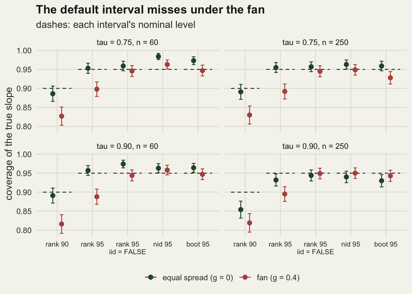
n_rep2  <- 2000      # a second, independent batch: default interval only
g_sweep <- c(0, 0.1, 0.2, 0.3, 0.4)
set.seed(3452)
batch2 <- do.call(rbind, lapply(g_sweep, function(g) {
  b_t <- q_slope(0.9, g)
  m <- t(replicate(n_rep2, {
    d <- sim_plots(250, g)
    ci <- suppressWarnings(rq.fit.br(cbind(1, d$open), d$growth, tau = 0.9,
                                     ci = TRUE))$coefficients[2, ]
    c(ci[2] <= b_t & b_t <= ci[3], ci[1])
  }))
  data.frame(g = g, coverage = mean(m[, 1]), sd_slope = sd(m[, 2]))
}))
batch2$mcse <- sqrt(batch2$coverage * (1 - batch2$coverage) / n_rep2)
k_flat4 <- which(cells$g == g_flat & cells$n == 250 & cells$tau == 0.9)
sd_first <- sd(raw[[k_flat4]][, 11])
cell4 <- cov_tab[cov_tab$g == g_flat & cov_tab$n == 250 & cov_tab$tau == 0.9, ]
fan_gap_se <- (0.9 - fan_def) / mcse_90
fan_r95 <- cov_tab$coverage[grid_rows & cov_tab$g == g_fan & cov_tab$arm == arms[2]]
fan_r90 <- cov_tab$coverage[grid_rows & cov_tab$g == g_fan & cov_tab$arm == arms[1]]
lift <- range(fan_r95 - fan_r90); short95 <- range(0.95 - fan_r95)
gap3 <- 0.9 - min(flat_def[1:3]); stopifnot(gap3 < 2 * mcse_90)
stopifnot(all(c(flat_def, batch2$coverage[1]) < 0.9))
fan_drop <- flat_def - fan_def          # same cell, equal spread minus fan
drop_b2 <- batch2$coverage[1] - batch2$coverage[5]
With equal spread, three of the four cells put the default interval at 0.886, 0.891 and 0.891, within 0.014 of its nominal 0.90, less than two Monte Carlo standard errors of 0.009. The fourth, 250 plots at the 0.9 quantile, came out at 0.854. Every interval in that cell sits below its level, the four ninety five per cent ones at 0.932, 0.944, 0.940, 0.930, and the slope estimates in it have a standard deviation of 0.221. The second batch in the chunk above draws 2000 fresh datasets for the same cell and five levels of g, scoring only the default: there the slope estimates have a standard deviation of 0.207 and the default covers 0.882, with a Monte Carlo standard error of 0.007. So with equal spread the default sits a little under its ninety per cent: all five estimates are below it.
Under the fan it covers between 0.816 and 0.830 in all four cells, 7.4 to 8.9 standard errors short of its own ninety per cent. Part of that is there without any fan: against the equal spread generator in the same cell, the fan costs a further 0.035 to 0.075 of coverage, the smallest in the cell with 250 plots at the 0.9 quantile, where the second batch puts it at 0.046. The shortfall is against the level the interval states, so it is not the ninety versus ninety five question; the equal spread assumption is being broken by the very feature the quantile regression was fitted to describe.
Asking for ninety five per cent with alpha = 0.05 keeps the same assumption. Under the fan it covers 0.898 and 0.892 at the 0.75 quantile with 60 and 250 plots, and 0.888 and 0.895 at the 0.9 quantile, against a nominal 0.95 and a Monte Carlo standard error of 0.007. The wider level adds 0.062 to 0.076 of coverage, and the interval still falls 0.052 to 0.062 short of 0.95.
rep_rows <- grid_rows & cov_tab$g == g_fan & cov_tab$arm %in% arms[3:5]
rep_rng <- function(a) range(cov_tab$coverage[rep_rows & cov_tab$arm == arms[a]])
nid_flat_60 <- cov_tab$coverage[grid_rows & cov_tab$g == g_flat & cov_tab$n == 60 &
                                cov_tab$arm == arms[4]]
unb <- cov_tab[cov_tab$arm == arms[3] & cov_tab$n_unbounded > 0, ]
unb_tot <- sum(unb$n_unbounded)
unb_max <- if (nrow(unb) > 0) max(unb$n_unbounded) else 0
nid_warn_share <- vapply(raw, function(m) mean(m[, 15] > 0), 0)
nid_k_max <- vapply(raw, function(m) max(m[, 15]), 0); k_worst <- which.max(nid_k_max)
m_w <- raw[[which.max(nid_warn_share)]]; nid_k_med <- median(m_w[m_w[, 15] > 0, 15])
unb_cell <- unb[which.max(unb$n_unbounded), ]
warn_cell <- cells[which.max(nid_warn_share), ]
min_rep <- min(cov_tab$coverage[rep_rows])
min_short <- min(c(0.9 - fan_r90, 0.95 - fan_r95))
stopifnot((nid_flat_60[1] - 0.95) / mcse_95 > 3, abs(nid_flat_60[2] - 0.95) < 2 * mcse_95,
          which.min(fan_drop) == 4)
gen_name <- function(g) if (g == g_fan) "fan" else if (g == g_flat) "equal spread" else
  sprintf("g = %.1f", g)
The three intervals that do not assume equal spread cover 0.944 to 0.949 (rank with iid = FALSE), 0.949 to 0.963 (nid) and 0.928 to 0.947 (pairs bootstrap) across the four fan cells. Kocherginsky, He and Mu 2005 compared the interval methods in quantreg and point out that approximations built on the iid error assumption are sensitive to even minor departures from it; the simulation here is one ecological case of that comparison, not a new result.
None of the three is free. With equal spread and 60 plots, nid covers 0.984 at the 0.75 quantile, well above its nominal 0.95, which means it is wider than it needs to be there; its 0.963 at the 0.9 quantile is within two Monte Carlo standard errors of 0.95. The rank interval with iid = FALSE returned a bound at the largest representable number, an interval that is in effect unbounded, in 21 of the datasets across all cells, 17 of them in the fan cell with 60 plots at the 0.90 quantile; those count as covering, and a reader would not accept them as an answer. The nid summary warned about non-positive local density estimates in up to 18.1 per cent of the datasets in a cell (the fan cell with 60 plots at the 0.90 quantile). The median warned fit there had 2 such plots out of 60, and the most in any single fit, in any cell, was 24 of 250 plots. The help page suggests considering the bootstrap when these estimates are a large proportion of the sample, so the warning is a reason to look at the count it reports, not only at whether it appears.
Why the equal spread interval is too short
The asymptotic variance of a quantile regression slope, set out in Koenker 2005, depends on the density of the errors at the fitted quantile, point by point. With equal spread that density is the same for every plot and one number describes it. Under the fan the density at the ninetieth percentile is high in the shaded plots, where the scatter is tight, and low in the open plots, where it is wide. Both ends of the gradient pull hardest on the slope, and the variance of the slope adds up what happens at the two ends, roughly the squared spread at each, so the wide open end dominates it. An equal spread method replaces the density plot by plot with its average over all plots, and that average, of one over the spread, is dominated by the tight shaded end. It treats the open plots as more precise than they are and so understates the variance. The nid sandwich estimates the density locally for each plot, and the pairs bootstrap resamples whole plots and never estimates it at all.
For this design the size of that error is arithmetic, not a simulation result. With many plots, the iid standard error of the slope divided by the correct one is the square root of the ratio of two variances: the equal spread formula, with one averaged density, over the sandwich of Koenker 2005, with the density plot by plot. The density of the gamma error at the quantile cancels, so the ratio depends neither on the error shape nor on tau, only on how the spread changes along the gradient and where the plots are.
asym_ratio <- function(g) {   # large-sample iid SE of the slope / correct SE
  x <- seq(0, 10, length.out = 10001); s <- 2.5 + g * (x - 5)   # density at quantile: f / s
  X <- cbind(1, x); J <- crossprod(X) / length(x)
  H <- crossprod(X / s, X) / length(x)                           # f cancels in the ratio
  sqrt(solve(J)[2, 2] / mean(1 / s)^2 / (solve(H) %*% J %*% solve(H))[2, 2])
}
asym <- vapply(g_sweep, asym_ratio, 0)
stopifnot(isTRUE(all.equal(asym[1], 1)), all(diff(asym) < 0), all(diff(diff(asym)) < 0))
For g of 0.0, 0.1, 0.2, 0.3, 0.4 the ratio is 1.00, 0.99, 0.96, 0.90, 0.80: nothing at first, then a shortfall that grows faster with every step of the fan. The simulated standard errors show the same thing without any interval. Each standard error method should match, on average, the actual spread of the slope estimates, their standard deviation across datasets. That standard deviation pools the one thousand datasets of the first batch with the two thousand of the second, drawn for the same five cells, because one thousand alone gave 0.221 with equal spread against 0.207 in the second batch.
se_tab <- do.call(rbind, lapply(which(cells$n == 250 & cells$tau == 0.9), function(k) {
  m <- raw[[k]]
  sd_2 <- batch2$sd_slope[abs(batch2$g - cells$g[k]) < 1e-9]
  sd_emp <- sqrt(((n_rep - 1) * sd(m[, 11])^2 + (n_rep2 - 1) * sd_2^2) /
                   (n_rep + n_rep2 - 2))   # pooled over both batches
  data.frame(g = cells$g[k], method = c("iid", "nid", "xy bootstrap"),
             ratio = colMeans(m[, 12:14]) / sd_emp, sd_emp = sd_emp)
}))
se_tab$method <- factor(se_tab$method, levels = c("iid", "nid", "xy bootstrap"))
r_se <- function(g, m) se_tab$ratio[se_tab$g == g & se_tab$method == m]
iid_rel <- r_se(g_fan, "iid") / r_se(g_flat, "iid")
stopifnot(abs(iid_rel - asym[5]) < 0.05, r_se(g_flat, "nid") > 1, r_se(g_fan, "nid") > 1)
With 250 plots at the 0.9 quantile, the average iid standard error is 0.92 times the actual standard deviation of the slope estimates with equal spread, and 0.73 times under the fan. At this sample size the iid estimate is 8 per cent low even with equal spread, and the fan multiplies it by a further 0.80; the arithmetic above gives 0.80. The nid standard error is 1.06 and 1.08 times, a little too large in both, and the bootstrap 1.03 and 1.05 times. The default rank interval is not built from the iid standard error, but it rests on the same equal spread assumption, and its coverage falls across the same sweep.
sw_tab <- cov_tab[cov_tab$n == 250 & cov_tab$tau == 0.9, ]
p_cov <- ggplot(sw_tab, aes(g, coverage, colour = arm)) +
  geom_hline(yintercept = c(0.90, 0.95), colour = te_body, linetype = "dashed",
             linewidth = 0.4) +
  geom_line(aes(linetype = arm), linewidth = 0.8) + geom_point(size = 1.8) +
  geom_point(data = batch2, aes(g, coverage), inherit.aes = FALSE, shape = 21,
             size = 2.6, stroke = 0.9, colour = te_rust, fill = te_paper) +
  scale_colour_manual(values = c(te_rust, te_gold, te_forest, te_forest, te_ink),
                      name = NULL) +
  scale_linetype_manual(values = c("solid", "solid", "22", "solid", "solid"),
                        name = NULL) +
  guides(colour = guide_legend(ncol = 2), linetype = guide_legend(ncol = 2)) +
  labs(x = "fan strength g", y = "coverage of the true slope",
       title = "Coverage", subtitle = "open circles: default, second batch") +
  theme_datasheet() + theme(legend.position = "bottom",
                            legend.text = element_text(size = 8.5))
p_se <- ggplot(se_tab, aes(g, ratio, colour = method)) +
  geom_hline(yintercept = 1, colour = te_body, linetype = "dashed", linewidth = 0.4) +
  geom_line(data = data.frame(g = g_sweep, ratio = asym), aes(g, ratio),
            inherit.aes = FALSE, colour = te_rust, linetype = "dotted", linewidth = 0.8) +
  geom_line(linewidth = 0.8) + geom_point(size = 1.8) +
  scale_colour_manual(values = c(te_rust, te_forest, te_ink), name = NULL) +
  labs(x = "fan strength g", y = "mean standard error / actual SD",
       title = "Standard errors", subtitle = "dashed: calibrated\ndotted: iid, large n") +
  theme_datasheet() + theme(legend.position = "bottom")
p_cov + p_se + plot_layout(widths = c(1.25, 1)) +
  plot_annotation(theme = theme_datasheet())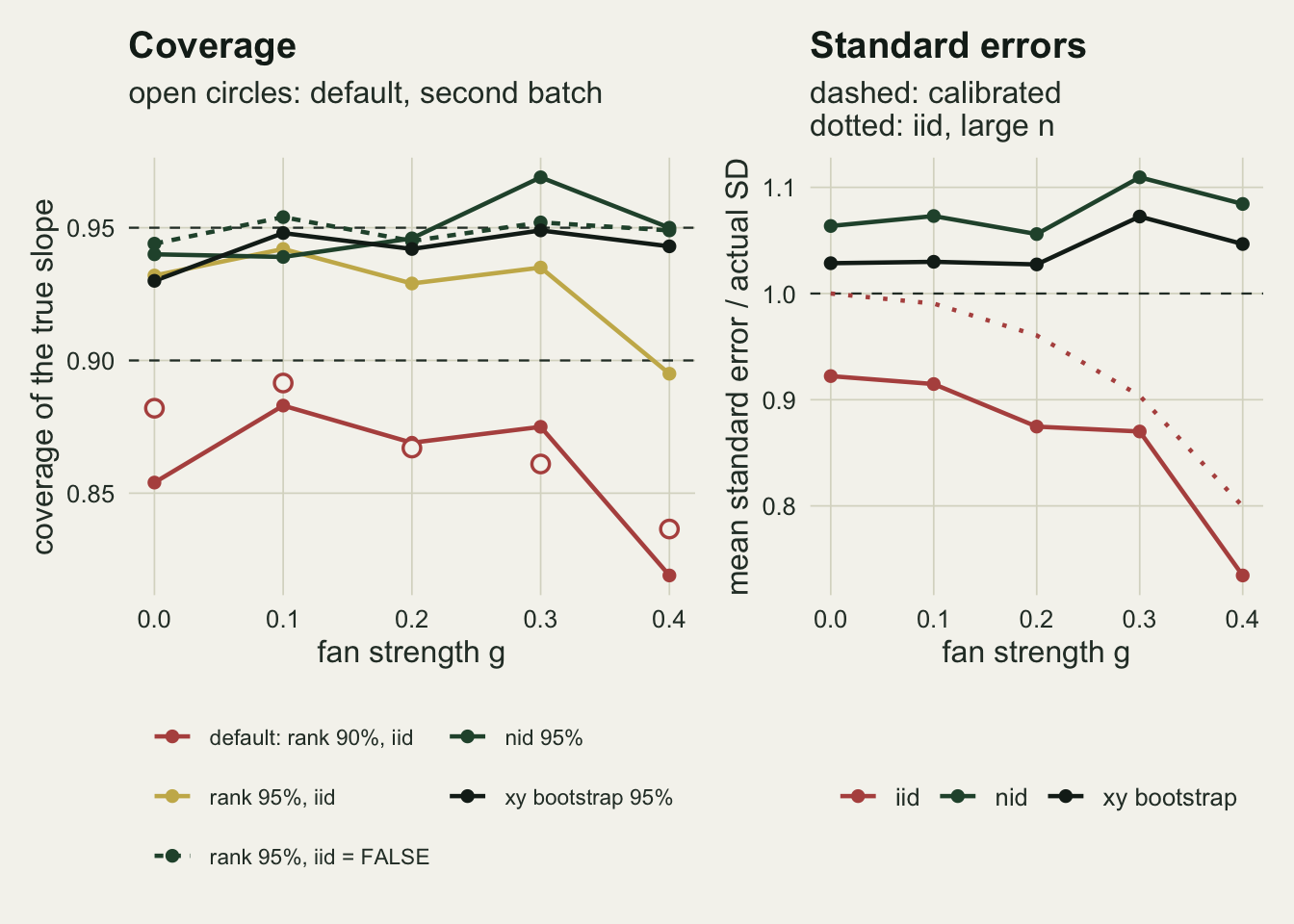
sw_def <- sw_tab$coverage[sw_tab$arm == arms[1]]
sw_g <- sw_tab$g[sw_tab$arm == arms[1]]
w_rel <- function(a, g = g_fan) sw_tab$width_med[sw_tab$g == g & sw_tab$arm == arms[a]] /
  sw_tab$width_med[sw_tab$g == g & sw_tab$arm == arms[2]]
spread_ratio <- (2.5 + 5 * g_sweep) / (2.5 - 5 * g_sweep)
b2 <- batch2$coverage
step_se <- abs(diff(b2)) / sqrt(head(batch2$mcse, -1)^2 + tail(batch2$mcse, -1)^2)
fall_se <- (b2[1] - b2[5]) / sqrt(batch2$mcse[1]^2 + batch2$mcse[5]^2)
stopifnot(which.min(sw_def[order(sw_g)]) == 5, which.min(b2) == 5, fall_se > 3)
Along the sweep the default covers 0.854, 0.883, 0.869, 0.875, 0.819 in the first batch and 0.882, 0.891, 0.867, 0.861, 0.836 in the second, for g of 0.0, 0.1, 0.2, 0.3, 0.4. Those values of g make the spread in the most open plots 1.0, 1.5, 2.3, 4.0, 9.0 times the spread in the most shaded ones. In both batches the default is lowest at g = 0.4. Neighbouring levels differ by at most 2.4 standard errors of a difference, so the shape of the curve between them is not resolved; the fall across the whole sweep is resolved: 0.046 in the second batch from g = 0 to g = 0.4, 4.1 standard errors of the difference. Repair costs width: in the fan with 250 plots at the 0.9 quantile, the median nid interval is 1.26 times as wide as the rank interval at ninety five per cent, the bootstrap 1.19 times and the rank interval with iid = FALSE 1.22 times. With equal spread the same ratios are 1.12, 1.07 and 1.02, so only the part beyond those is uncertainty that the equal spread interval left out because of the fan.
What to report
Name the interval method and its level. “95 per cent confidence interval from quantreg” is not enough, because the package prints a ninety per cent rank interval by default below 1001 observations, a nid standard error above it, and neither the column headings nor the output say which assumption was used. A sentence such as “rank inversion interval, alpha = 0.05, iid = FALSE” or “xy pairs bootstrap, 200 resamples” is enough for a reader to check it.
If the reason for fitting a quantile regression was a fan, a wedge or a limiting factor, do not use an interval that assumes equal spread. In the fan cells of this simulation the three that do not assume it covered at least 0.928 against a nominal 0.95, and the two that do assume it fell at least 0.052 short of their own levels.
Quote the sample size alongside the method. The switch at 1001 rows means that the same script run on a larger dataset silently changes its interval method, from a ninety per cent rank interval to a standard error, t value and p value computed by nid.
Look at the fan before choosing. A plot of the residuals of a median fit against the covariate shows whether the spread changes, and so whether the default is defensible for the data in hand; the post on checking a quantile regression covers the other checks a fit needs before any interval is worth reporting.
Honest limits
The simulation uses one error shape, a gamma with shape two, and one form of changing spread, linear in the covariate, with a single covariate spread evenly along the gradient. The conditional quantiles are exactly linear, so every interval here is aimed at a slope that exists. A fan that is not linear, or a covariate with a few isolated extreme plots, changes which plots pull hardest on the slope, and so the undercoverage, and the sizes measured here do not transfer without rerunning the code.
The quantile levels stop at 0.9 and the sample sizes at 60 and 250. At the 0.95 or 0.99 level, or with fewer than the 60 plots tested here, the nid sparsity estimate has very few points to work with and the pairs bootstrap resamples the same handful of observations near the top, which is the problem Checking a quantile regression describes. Nothing here shows that nid or the bootstrap is safe there, and it should not be read that way.
The bootstrap used 200 resamples and a normal type interval from its standard error, not a percentile interval, and only the pairs scheme; the wild and Markov chain marginal bootstraps that boot.rq also offers were not run. Its coverage was measured on one thousand datasets per cell, so its Monte Carlo standard error is about 0.007 near ninety five per cent, and differences of that size between the three repair methods are not findings.
Only the slope was scored. The intercept, a joint interval for several quantiles, and a test of whether two quantile slopes differ, which is what Heteroscedasticity and limiting factors uses to show that the fan is real, each have their own coverage and were not measured.
The simulation took 130 seconds on the machine that knitted this page, and the version checks are tied to quantreg 6.1. The guard reads the switch from the source of summary.rq rather than from its help page, so a change in a later version stops the knit.
References
Cade BS, Noon BR 2003 Frontiers in Ecology and the Environment 1(8):412-420 (10.1890/1540-9295(2003)001[0412:AGITQR]2.0.CO;2)
Koenker R 1994 Asymptotic Statistics (Contributions to Statistics), Physica-Verlag:349-359 (10.1007/978-3-642-57984-4_29)
Koenker R, Machado JAF 1999 Journal of the American Statistical Association 94(448):1296-1310 (10.1080/01621459.1999.10473882)
Hendricks W, Koenker R 1992 Journal of the American Statistical Association 87(417):58-68 (10.1080/01621459.1992.10475175)
Kocherginsky M, He X, Mu Y 2005 Journal of Computational and Graphical Statistics 14(1):41-55 (10.1198/106186005X27563)
Koenker R 2005 Quantile Regression (ISBN 978-0-521-84573-1)