library(nlme)
library(ggplot2)

set.seed(52)
k <- 4; m <- 10; ntank <- 2 * k
tank_eff  <- rnorm(ntank, 0, 1)                  # tanks genuinely differ
grp_tank  <- rep(c("C", "T"), each = k)          # treatment assigned at TANK level
fish_tank <- rep(1:ntank, each = m)
y <- 10 + tank_eff[fish_tank] + rnorm(ntank * m, 0, 1)   # no treatment term anywhere
dat <- data.frame(y, tank = factor(fish_tank), grp = factor(grp_tank[fish_tank]))Pseudoreplication and false positives in ecology
R
mixed models
experimental design
ecology tutorial
Treating repeated measurements as independent replicates inflates false positives. A simulation shows the cost, and how aggregating or a mixed model fixes it.
You apply a treatment to four tanks and a control to four others, measure ten fish in each tank, and run a t test on all eighty fish. It comes back significant. You have just committed pseudoreplication, and your p value is close to meaningless. The eighty fish are not eighty independent pieces of evidence about the treatment; they are eight tanks worth, and the ten fish inside a tank are more like each other than they are like fish in another tank. Counting them as independent inflates your sample size on paper and your false-positive rate in practice.
Hurlbert gave this its name in 1984 and found it in a remarkable fraction of the literature: of 176 experimental studies he examined, 27 percent contained pseudoreplication, and among those that used inferential statistics at all the figure was 48 percent. Four decades on it remains one of the most common analysis errors in ecology, precisely because the broken analysis looks so reasonable and reports such satisfying p values.
His definition is worth stating plainly: pseudoreplication is testing for a treatment effect using an error term that does not match the scale at which the treatment was applied. The treatment was applied to tanks, so tanks are the unit of replication; the fish are subsamples. It comes in a few standard flavours. Simple pseudoreplication treats subsamples within an experimental unit as replicates, the tank example above. Temporal pseudoreplication treats repeated measurements of the same unit over time as independent. Sacrificial pseudoreplication pools away the unit structure before testing. All three share one root: the analysis pretends there is more independent information than the design actually delivered.
One false positive, dissected
Here is a single dataset with no treatment effect at all. Eight tanks, four assigned to each group, ten fish each. The only structure is that tanks differ from one another (a random tank effect), exactly as real tanks do.
The clustering is obvious once you plot it: fish within a tank sit together, and the tanks are scattered. The treatment and control clouds overlap completely, because there is no effect.
tm <- aggregate(y ~ tank + grp, dat, mean)
ggplot(dat, aes(tank, y, colour = grp)) +
  geom_jitter(width = 0.15, height = 0, alpha = 0.5, size = 1.6) +
  geom_point(data = tm, aes(tank, y), size = 4.5, shape = 18) +
  scale_colour_manual(values = c(C = "#275139", T = "#cda23f"),
                      labels = c("control", "treatment"), name = NULL) +
  labs(x = "tank", y = "measurement") +
  theme_minimal(base_size = 12) +
  theme(panel.grid.minor = element_blank(),
        plot.background = element_rect(fill = "#f5f4ee", colour = NA),
        panel.background = element_rect(fill = "#f5f4ee", colour = NA))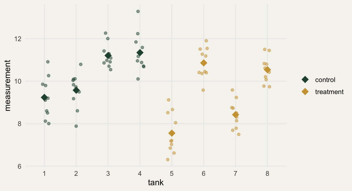
Now the two analyses. The naive one treats every fish as a replicate; the honest one collapses each tank to its mean and tests the eight tank means.
m_naive <- lm(y ~ grp, data = dat)                       # 80 "replicates": WRONG
m_tank  <- lm(y ~ grp, data = aggregate(y ~ tank + grp, dat, mean))  # 8 tanks: correct
c(naive_estimate = round(coef(m_naive)["grpT"], 3),
  naive_df       = m_naive$df.residual,
  naive_p        = round(summary(m_naive)$coefficients["grpT", "Pr(>|t|)"], 4))
naive_estimate.grpT naive_df naive_p
-0.9970 78.0000 0.0025 c(tank_estimate = round(coef(m_tank)["grpT"], 3),
tank_df = m_tank$df.residual,
tank_p = round(summary(m_tank)$coefficients["grpT", "Pr(>|t|)"], 3))tank_estimate.grpT tank_df tank_p
-0.997 6.000 0.345 The two models report the same estimated difference, about -1.0, because pseudoreplication does not bias the point estimate. What differs is everything used to judge it. The naive model claims 78 residual degrees of freedom and returns p = 0.0025, a confident false positive. The correct model has 6 degrees of freedom (eight tanks minus two group means) and returns p = 0.34, no effect, which is the truth. The inflated denominator degrees of freedom is the signature of the error: the naive model thinks it has ten times the information it really has.
Is that just an unlucky dataset?
No. Run the same null design thousands of times and count how often each analysis falsely declares significance. If a test is valid, it should reject a true null exactly 5 percent of the time.
set.seed(7)
sim_once <- function(k = 4, m = 10, sd_tank = 1, sd_resid = 1, mu = 10) {
  ntank <- 2 * k
  tank_eff  <- rnorm(ntank, 0, sd_tank)
  grp_tank  <- rep(c("C", "T"), each = k)
  fish_tank <- rep(1:ntank, each = m)
  y <- mu + tank_eff[fish_tank] + rnorm(ntank * m, 0, sd_resid)   # null: no effect
  grp_fish <- factor(grp_tank[fish_tank])
  p_naive <- t.test(y ~ grp_fish)$p.value                        # every fish a replicate
  tank_mean <- tapply(y, fish_tank, mean)
  p_tank <- t.test(tank_mean ~ factor(grp_tank))$p.value         # tanks as replicates
  c(p_naive, p_tank)
}
res <- t(replicate(2000, sim_once()))
c(naive_false_positive = round(mean(res[, 1] < 0.05), 3),
  tank_false_positive  = round(mean(res[, 2] < 0.05), 3))
naive_false_positive tank_false_positive
0.447 0.040 The naive analysis rejects the true null about 45 percent of the time. Nearly half of all “significant” results from this design would be false. The tank-level analysis sits at 4 percent, right where a valid test should be. This is not a subtle bias; it is a test that is wrong roughly nine times more often than it advertises.
rd <- data.frame(
  method = factor(c("naive (per fish)", "tank means"),
                  levels = c("naive (per fish)", "tank means")),
  rate = c(mean(res[, 1] < 0.05), mean(res[, 2] < 0.05)))
ggplot(rd, aes(method, rate, fill = method)) +
  geom_col(width = 0.55) +
  geom_hline(yintercept = 0.05, linetype = "dashed", colour = "#16241d", linewidth = 0.7) +
  annotate("text", x = 1.5, y = 0.115, label = "nominal 0.05",
           colour = "#16241d", size = 3.3, family = "mono") +
  geom_text(aes(label = sprintf("%.0f%%", 100 * rate)), vjust = -0.4,
            colour = "#16241d", size = 4.4, family = "mono") +
  scale_fill_manual(values = c("naive (per fish)" = "#b5534e", "tank means" = "#275139"),
                    guide = "none") +
  scale_y_continuous(limits = c(0, 0.55), labels = function(x) paste0(100 * x, "%")) +
  labs(x = NULL, y = "false-positive rate") +
  theme_minimal(base_size = 12) +
  theme(panel.grid.minor = element_blank(),
        plot.background = element_rect(fill = "#f5f4ee", colour = NA),
        panel.background = element_rect(fill = "#f5f4ee", colour = NA))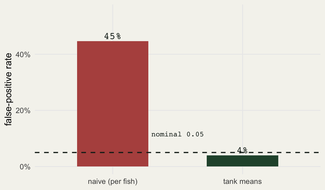
The fix
The principle is one sentence: your sample size is the number of independent experimental units, not the number of measurements. With eight tanks you have eight replicates, whatever the fish count.
The simplest valid analysis is to aggregate each unit to a single value and test those, which is what m_tank did. It is transparent, it is correct for balanced designs, and it needs no special machinery. Its only cost is that it discards the within-tank information entirely.
The more general fix is a mixed model with a random effect for the experimental unit, which keeps every fish in the model while still attributing the right amount of information to each level.
m_mixed <- lme(y ~ grp, random = ~1 | tank, data = dat)
round(summary(m_mixed)$tTable["grpT", c("Value", "p-value")], 3)
Value p-value
-0.997 0.345 round(as.numeric(VarCorr(m_mixed)[, "StdDev"]), 3) # SD: tank, then residual[1] 1.353 0.796The mixed model returns p = 0.34, the same honest verdict as the tank means, and in a balanced design like this the two are mathematically equivalent. What it adds is the variance breakdown: a tank-level standard deviation of 1.35 against a residual of 0.80. That implies an intraclass correlation near 0.74, meaning most of the variation lives between tanks, which is exactly why ignoring tanks was so damaging. The mixed model earns its keep in the harder cases the aggregation cannot handle: unbalanced subsampling, within-unit covariates, crossed random effects, and non-normal responses through its generalised cousin. Bolker and colleagues give the practical roadmap.
A necessary caveat
The concept can be over-applied, and a reflexive accusation of pseudoreplication has sometimes buried perfectly good ecology. Davies and Gray make the case that natural experiments, landscape-scale manipulations, and rare events are often unreplicable by their nature, and that refusing to analyse them is its own kind of error. Two points from that debate are worth carrying. First, confounding and pseudoreplication are different problems; a single treated site next to several controls may be confounded, but that is an argument about inference and causation, not a licence to inflate degrees of freedom. Second, the answer to non-independence is usually to model it, with random effects, spatial or temporal correlation structures, and an honest accounting of the real replication, rather than to abandon the data. The sin is not having correlated data; it is pretending you do not.
Practical guidance
Identify the experimental unit before you touch the statistics: it is whatever the treatment was independently applied to. Count your replicates at that level, and let that be your n. If you have subsamples, either aggregate them to the unit and analyse the units, or fit a mixed model with a random effect for the unit; never feed the raw subsamples to a test that assumes independence. Treat repeated measurements on the same unit as the temporal pseudoreplication they are, with a unit random effect or a correlation structure. And read the degrees of freedom your model reports: if they look far larger than your number of independent units, the model is almost certainly counting subsamples as replicates, and the p value beneath them is not to be trusted.
References
Hurlbert 1984 Ecological Monographs 54(2):187-211 (10.2307/1942661)
Bolker et al. 2009 Trends in Ecology and Evolution 24(3):127-135 (10.1016/j.tree.2008.10.008)
Davies and Gray 2015 Ecology and Evolution 5(22):5295-5304 (10.1002/ece3.1782)