library(ape)
library(nlme)
library(ggplot2)

te_paper <- "#f5f4ee"; te_ink   <- "#16241d"; te_body <- "#2c3a31"
te_faint <- "#5d6b61"; te_sage  <- "#93a87f"; te_rust <- "#b5534e"
te_line  <- "#dad9ca"; te_green <- "#2f8f63"; te_gold <- "#cda23f"

theme_te <- function(base_size = 12) {
  theme_minimal(base_size = base_size) +
    theme(
      plot.background  = element_rect(fill = te_paper, colour = NA),
      panel.background = element_rect(fill = te_paper, colour = NA),
      panel.grid.major = element_line(colour = te_line, linewidth = 0.3),
      panel.grid.minor = element_blank(),
      axis.text  = element_text(colour = te_body),
      axis.title = element_text(colour = te_ink),
      plot.title = element_text(colour = te_ink, face = "bold"),
      strip.text = element_text(colour = te_ink, face = "bold")
    )
}Phylogenetic generalised least squares
R
ape
nlme
phylogenetics
comparative methods
ecology tutorial
PGLS in R with ape and nlme: why ordinary regression across related species inflates false positives, and how corBrownian and corPagel fix the problem.
Regressing one trait on another across species looks like ordinary regression, but the observations break its central assumption. Related species are not independent: they inherited much of their similarity from common ancestors, so a sample of fifty species carries far fewer than fifty independent pieces of evidence. Ordinary least squares does not know this, treats every species as a fresh observation, and reports standard errors that are too small. The result is a flood of significant relationships that are not real.
Phylogenetic generalised least squares, PGLS, is the standard cure. It is ordinary regression with one change: the residuals are allowed to be correlated, with the correlation set by the tree. Species that share a long stretch of history are expected to have similar residuals, and the model accounts for that when it weighs the evidence. In R it is a one-line change from lm to gls, using ape for the tree structure and nlme for the fitting.
Setup
The problem, in numbers
The cleanest way to see the damage is to simulate data with no relationship at all and count how often each method claims one. We take a single 40-species tree and, one thousand times over, evolve two traits along it independently by Brownian motion. Because the traits are simulated separately, the true slope between them is zero. Any significant result is a false positive.
set.seed(2024)
tree <- rcoal(40)
tree$tip.label <- sprintf("t%02d", 1:40)

nsim <- 1000
p_ols <- p_pgls <- numeric(nsim)
set.seed(2024)
for (i in seq_len(nsim)) {
  xi <- rTraitCont(tree, "BM", sigma = 1)
  yi <- rTraitCont(tree, "BM", sigma = 1)   # evolved independently of xi
  di <- data.frame(sp = tree$tip.label, x = xi[tree$tip.label], y = yi[tree$tip.label])
  p_ols[i]  <- summary(lm(y ~ x, data = di))$coef[2, 4]
  fit_pgls  <- gls(y ~ x, data = di, correlation = corBrownian(1, tree, form = ~sp))
  p_pgls[i] <- summary(fit_pgls)$tTable[2, 4]
}

c(ols_false_positive  = mean(p_ols  < 0.05),
  pgls_false_positive = mean(p_pgls < 0.05))
ols_false_positive pgls_false_positive
0.541 0.048 Ordinary regression flags a significant slope in 54% of these null datasets, more than ten times the 5% you signed up for when you chose that threshold. PGLS, which knows the traits evolved on a tree, sits at 4.8%, right where a valid test should be. The inflation is not a quirk of one dataset; it is what ordinary regression does whenever the residuals carry phylogenetic structure.
dfp <- rbind(data.frame(method = "ordinary least squares", p = p_ols),
             data.frame(method = "PGLS (Brownian)",        p = p_pgls))
dfp$method <- factor(dfp$method, levels = c("ordinary least squares", "PGLS (Brownian)"))
ggplot(dfp, aes(p)) +
  geom_histogram(breaks = seq(0, 1, 0.05), fill = te_sage, colour = te_paper, linewidth = 0.2) +
  geom_vline(xintercept = 0.05, colour = te_rust, linewidth = 0.8, linetype = "22") +
  facet_wrap(~method) +
  labs(x = "p-value for the slope (true slope is zero)", y = "count of datasets",
       title = "A valid test spreads p-values evenly") +
  theme_te(12)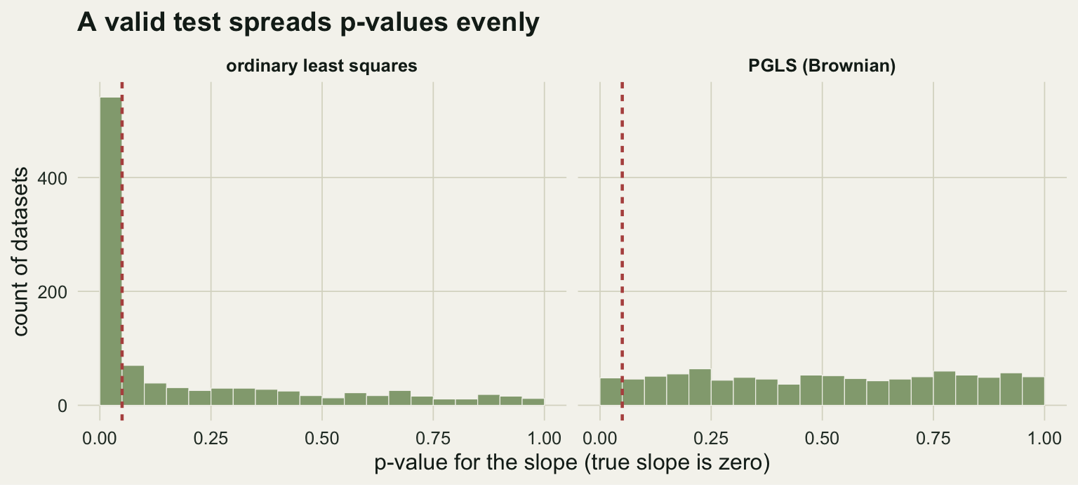
Fitting PGLS, and estimating how tree-like the residuals are
The simulation used corBrownian, which assumes the residuals follow Brownian motion exactly. That was the right choice there because the traits were built that way, but real data rarely commit so fully. A more honest option is corPagel, which multiplies the off-diagonal covariances by a parameter lambda and estimates it alongside the slope. Lambda of 1 is strict Brownian motion; lambda of 0 is ordinary regression with independent residuals; values in between say the residuals are partly, but not entirely, tree-like.
We build one dataset with a genuine relationship (a true slope of 0.6) and residuals that are only moderately phylogenetic, then fit all three models.
sim_pagel <- function(phy, lambda, sigma2 = 1) {
  V <- vcv(phy); Vl <- V * lambda; diag(Vl) <- diag(V)
  MASS::mvrnorm(1, rep(0, nrow(V)), sigma2 * Vl)
}
set.seed(101); tr <- rcoal(60); tr$tip.label <- sprintf("s%02d", 1:60)
set.seed(102); x <- sim_pagel(tr, 0.9)
set.seed(103); y <- 0.6 * x + sim_pagel(tr, 0.5, sigma2 = 1)
d <- data.frame(sp = tr$tip.label, x = x[tr$tip.label], y = y[tr$tip.label])

m_ols   <- gls(y ~ x, data = d, method = "ML")
m_bm    <- gls(y ~ x, data = d, correlation = corBrownian(1, tr, form = ~sp), method = "ML")
m_pagel <- gls(y ~ x, data = d, correlation = corPagel(0.5, tr, form = ~sp), method = "ML")
lambda_hat <- as.numeric(coef(m_pagel$modelStruct$corStruct, unconstrained = FALSE))

rbind(
  ols   = c(slope = coef(m_ols)[2],   AIC = AIC(m_ols)),
  brown = c(slope = coef(m_bm)[2],    AIC = AIC(m_bm)),
  pagel = c(slope = coef(m_pagel)[2], AIC = AIC(m_pagel)))
slope.x AIC
ols 0.7248915 224.7017
brown 0.4569170 288.7780
pagel 0.4607742 220.0637The estimated lambda is 0.55, squarely between the extremes: the residuals are about half as tree-like as strict Brownian motion. That matters for the answer. Ordinary regression gives a slope of 0.72 and strict Brownian gives 0.46, both above the true 0.6, while the Pagel fit lands at 0.46, closest to the generating value. By AIC the Pagel model wins, and strict Brownian is the worst of the three, a useful reminder that the wrong correlation structure can hurt more than no correction at all. Estimating lambda lets the data set the dial rather than assuming it.
rng <- range(d$x); mx <- mean(d$x); my <- mean(d$y)
line_at <- function(b) data.frame(x = rng, y = my + b * (rng - mx))
lines_df <- rbind(
  cbind(model = "true (0.6)",              line_at(0.6)),
  cbind(model = "ordinary least squares",  line_at(coef(m_ols)[2])),
  cbind(model = "Brownian (lambda = 1)",   line_at(coef(m_bm)[2])),
  cbind(model = sprintf("Pagel (lambda = %.2f)", lambda_hat), line_at(coef(m_pagel)[2])))
lev <- c("true (0.6)", "ordinary least squares", "Brownian (lambda = 1)",
         sprintf("Pagel (lambda = %.2f)", lambda_hat))
lines_df$model <- factor(lines_df$model, levels = lev)
ggplot(d, aes(x, y)) +
  geom_point(colour = te_faint, alpha = 0.6, size = 1.8) +
  geom_line(data = lines_df, aes(colour = model, linetype = model), linewidth = 0.9) +
  scale_colour_manual(values = c(te_ink, te_rust, te_gold, te_green)) +
  scale_linetype_manual(values = c("22", "solid", "solid", "solid")) +
  labs(x = "trait x", y = "trait y", colour = NULL, linetype = NULL,
       title = "Estimating lambda sets the right amount of correction") +
  guides(colour = guide_legend(nrow = 2), linetype = guide_legend(nrow = 2)) +
  theme_te(12) + theme(legend.position = "bottom")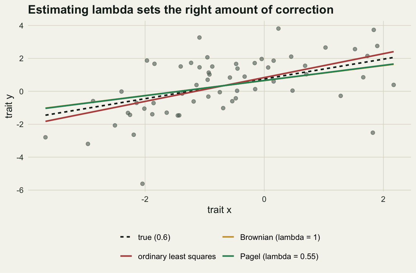
Reading it
PGLS earns its keep because it fixes the standard errors, not because it always moves the slope a lot. Under the null, as the simulation showed, the slope is near zero either way; what ordinary regression gets wrong is the uncertainty, and that is what produces false positives. With a real signal the slope can shift too, as it did here, but the reliable inference is the point.
A few practical notes. Prefer corPagel to corBrownian unless you have a strong reason to fix the model, since letting lambda float protects you when the residuals are less tree-like than Brownian motion. Lambda applies to the residuals of the regression, not to either trait on its own, so it is not the same as phylogenetic signal in a single trait; a trait can be strongly conserved while the residuals of a good model are not. And the whole apparatus assumes the tree and its branch lengths are roughly correct, so a badly resolved phylogeny will still mislead. When lambda comes out near 1, the fit coincides with independent contrasts, which is a good sanity check that the two routes agree.
References
- Grafen 1989 Philosophical Transactions of the Royal Society B 326(1233):119-157 (10.1098/rstb.1989.0106)
- Martins & Hansen 1997 The American Naturalist 149(4):646-667 (10.1086/286013)
- Freckleton, Harvey & Pagel 2002 The American Naturalist 160(6):712-726 (10.1086/343873)
- Revell 2010 Methods in Ecology and Evolution 1(4):319-329 (10.1111/j.2041-210X.2010.00044.x)
- Symonds & Blomberg 2014, in Garamszegi (ed.) Modern Phylogenetic Comparative Methods and Their Application in Evolutionary Biology, Springer (ISBN 978-3-662-43549-6)