---
title: "ordisurf vs envfit: nonlinear gradients in R"
description: "envfit draws one straight arrow assuming a single direction of increase; for a humped variable it points nowhere. Fit a smooth GAM surface with ordisurf in R."
date: "2026-05-02 15:00"
categories: [R, ordination, gradient analysis, vegan, ecology tutorial]
image: thumbnail.png
image-alt: "An NMDS ordination with ordisurf contours showing a central hump in elevation, beside a short envfit arrow that points nowhere useful."
---
The [envfit and PERMANOVA tutorial](../envfit-and-permanova/) fit environmental variables to an ordination as arrows. An arrow is a straight line: it says the variable increases steadily in one direction across the ordination and decreases in the opposite one. That is a strong assumption, and for many environmental variables it is wrong. Elevation, soil pH, and disturbance often have a *unimodal* shape over the ordination: the variable peaks somewhere in the middle of the compositional gradient and falls away towards both ends, so it climbs in one direction across half the picture and drops in the same direction across the other half. There is no single direction of increase for an arrow to point along, and `envfit` quietly reports almost nothing.
`ordisurf()` is the fix. Instead of a vector, it fits a smooth surface, a generalised additive model (Wood 2017), over the ordination and draws it as contour lines. A surface can bend, peak, and curve, so it captures structure that a straight arrow cannot. This post fits both methods to the same ordination, with one monotone variable and one humped variable, and shows exactly where the arrow succeeds and where it fails.
## Two variables, two shapes
The community sits on two latent gradients, the stronger of which drives most of the species turnover, so an NMDS recovers it as the first axis. Onto that we attach two environmental variables with deliberately different shapes. Moisture increases steadily along the primary gradient: monotone, the kind of variable an arrow is built for. Elevation peaks in the middle of the gradient and falls off toward both ends: a symmetric hump.
```{r}
#| label: data
#| message: false
#| warning: false
library(vegan)
library(mgcv)
library(ggplot2)
te_canvas <- theme(plot.background  = element_rect(fill = "#f5f4ee", colour = NA),
                   panel.background = element_rect(fill = "#f5f4ee", colour = NA))

set.seed(24)

n  <- 80
g1 <- runif(n, -2, 2)       # primary gradient: most turnover
g2 <- runif(n, -1.2, 1.2)   # weaker secondary gradient

# 18 species with 2D Gaussian niches
n_sp <- 18
o1 <- runif(n_sp, -2.2, 2.2); o2 <- runif(n_sp, -1.3, 1.3)
w1 <- 0.9; w2 <- 0.8; peak <- 22
lambda <- matrix(0, n, n_sp)
for (j in seq_len(n_sp))
  lambda[, j] <- peak * exp(-((g1 - o1[j])^2)/(2*w1^2) - ((g2 - o2[j])^2)/(2*w2^2))
comm <- matrix(rpois(length(lambda), lambda), nrow = n)
colnames(comm) <- paste0("sp", sprintf("%02d", seq_len(n_sp)))

# moisture: monotone in the primary gradient (an arrow should work)
moisture  <- 50 + 12 * g1 + rnorm(n, 0, 6)
# elevation: humped in the primary gradient (an arrow should fail)
elevation <- 400 - 70 * g1^2 + rnorm(n, 0, 20)

c(moisture_vs_g1 = cor(moisture, g1), elevation_vs_g1 = cor(elevation, g1))
```
The two correlations with the underlying gradient tell the whole story in advance. Moisture correlates near 0.9 with the primary gradient. Elevation correlates near zero, not because it is unrelated but because a symmetric hump has no linear trend: every rise on the left is cancelled by a matching fall on the right. A method that only looks for linear trend will see moisture clearly and elevation not at all.
## The ordination and the linear fit
Run the NMDS, then fit both variables with `envfit`.
```{r}
#| label: nmds-envfit
#| message: false
#| warning: false
set.seed(7)
mds <- metaMDS(comm, distance = "bray", k = 2, trymax = 100,
               autotransform = FALSE, trace = FALSE)

set.seed(42)
ef <- envfit(mds, data.frame(moisture = moisture, elevation = elevation),
             permutations = 999)
ef
```
The stress is low, so the two-dimensional picture is trustworthy. The `envfit` table splits the two variables cleanly. Moisture gets a large r-squared (near 0.81) and a significant p-value: the arrow is real and worth drawing. Elevation gets an r-squared near 0.03 and a non-significant p-value. Taken at face value, `envfit` says elevation has no relationship with the ordination. That conclusion is wrong, and the next step shows why.
## The smooth surface
`ordisurf()` fits a GAM smoother over the ordination scores and returns the fitted surface. Call it with `plot = FALSE` to keep the object without drawing the base graphic, then read the model summary.
```{r}
#| label: ordisurf
#| results: hold
os_moist <- ordisurf(mds ~ moisture,  plot = FALSE)
os_elev  <- ordisurf(mds ~ elevation, plot = FALSE)

summary(os_elev)
```
Look at the deviance explained for elevation: about 86%. The smooth term is significant at p below 0.001. The variable that `envfit` called nothing explains the large majority of the surface once you let the fit bend. Putting the two methods side by side makes the disagreement concrete.
Read that p-value with one qualification. `ordisurf()` does not hand the smooth to `mgcv::gam()` at gam's own defaults: it sets `select = TRUE`, which adds a second penalty on the part of the basis that the usual wiggliness penalty cannot touch, so the whole surface can be shrunk away to a flat plane. That is sensible behaviour for a plotting helper, and mgcv's help page for `summary.gam` says in as many words that the p-value approximation gets cruder for a term that can be penalised to zero. How much cruder is measurable on this very ordination. Shuffle the elevation values across the sites: the variable keeps its distribution, since it is the same set of numbers in a different order, but whatever tie it had to composition is gone. Then count how often the smooth is still called significant.
```{r}
#| label: ordisurf-null
#| message: false
#| warning: false
set.seed(4223)
reps <- 1000
perm_p <- t(replicate(reps, {
  shuffled <- sample(elevation)          # same values, no link to composition
  c(default = summary(ordisurf(mds, shuffled, plot = FALSE))$s.table[1, "p-value"],
    nosel   = summary(ordisurf(mds, shuffled, plot = FALSE,
                               select = FALSE))$s.table[1, "p-value"])
}))
os_null <- colMeans(perm_p < 0.05)
round(c(os_null, mc_se = sqrt(os_null * (1 - os_null) / reps)), 3)
```
A variable with no relationship to the community at all clears the 0.05 line about `r round(100 * os_null[["default"]])` per cent of the time under the default call, and about `r round(100 * os_null[["nosel"]])` per cent when the same shuffles are refitted with `select = FALSE`, which is where a calibrated test belongs. The shrinkage penalty, not the ordination and not the smoothing basis, is what roughly doubles the rate; the Monte Carlo error printed beside the two rates says the gap between them is real. Elevation here is nowhere in that territory, and neither is any surface whose deviance explained runs into the eighties. A marginal one is a different matter: refit it with `select = FALSE` before you believe the stars. Shrinkage is not the only way a smooth's p-value goes anti-conservative either; sharing information between two smooths does the same thing to the standard errors, which is the subject of [concurvity in additive models](../concurvity-in-additive-models/).
```{r}
#| label: compare
sm_m <- summary(os_moist); sm_e <- summary(os_elev)
data.frame(
  variable          = c("moisture", "elevation"),
  shape             = c("monotone", "humped"),
  envfit_r2         = round(ef$vectors$r, 3),
  envfit_p          = ef$vectors$pvals,
  ordisurf_dev_expl = round(100 * c(sm_m$dev.expl, sm_e$dev.expl), 1),
  ordisurf_edf      = round(c(sm_m$s.table[1, "edf"], sm_e$s.table[1, "edf"]), 2),
  row.names = NULL
)
```
For moisture the two methods agree: high envfit r-squared, high ordisurf deviance explained. The arrow and the surface tell the same story because the variable really does climb in one direction. For elevation they part company completely: envfit near zero, ordisurf near 86%. Notice that both surfaces carry a high effective degrees of freedom (`edf` near 6.7), not just the humped one. That is worth understanding: the NMDS embedding itself is curved, so even a monotone variable needs a slightly wavy surface to fit well in ordination space. A high `edf` flags that a straight arrow is a simplification; it does not by itself tell you the arrow will fail. What makes the arrow fail for elevation specifically is that the response is non-monotone, so no single direction summarises it.
## Drawing the surface
To put the surface in a ggplot rather than the base-graphics default, pull the fitted grid out of the `ordisurf` object. One trap worth flagging: `ordiArrowMul()`, the helper that scales `envfit` arrows to the plot, returns `Inf` when there is no active base plot, so under ggplot you scale the arrow by hand instead.
```{r}
#| label: fig-elev
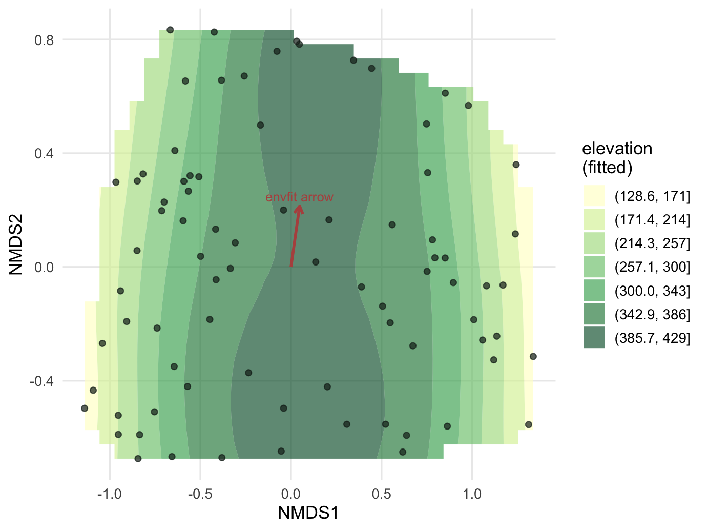
#| fig-cap: "Elevation as an ordisurf surface. The contours reveal a central hump that the short, non-significant envfit arrow completely misses."
#| fig-alt: "An NMDS ordination overlaid with filled ordisurf contours forming a central elevation hump, with site points and a short envfit arrow that starts inside the hump and points roughly up the second axis, along the ridge rather than across it."
#| fig-width: 7.2
#| fig-height: 5.4
# tidy the fitted surface grid
surf_df <- function(os) {
  g <- expand.grid(NMDS1 = os$grid$x, NMDS2 = os$grid$y)
  g$z <- as.vector(os$grid$z)
  g[!is.na(g$z), ]
}
site <- as.data.frame(scores(mds, display = "sites"))

# manual arrow scaling (ordiArrowMul returns Inf under ggplot)
arr <- as.data.frame(scores(ef, "vectors")); arr$var <- rownames(arr)
mul <- 0.85 * max(abs(site[, c("NMDS1", "NMDS2")])) /
              max(sqrt(rowSums(arr[, 1:2]^2)))
arr_e <- arr[arr$var == "elevation", ]

ggplot() +
  geom_contour_filled(data = surf_df(os_elev), aes(NMDS1, NMDS2, z = z),
                      alpha = 0.65, bins = 8) +
  geom_point(data = site, aes(NMDS1, NMDS2), colour = "#16241d",
             size = 1.7, alpha = 0.7) +
  geom_segment(data = arr_e, aes(0, 0, xend = NMDS1*mul, yend = NMDS2*mul),
               arrow = arrow(length = unit(0.22, "cm")),
               linewidth = 1, colour = "#b5534e") +
  geom_text(data = arr_e, aes(NMDS1*mul, NMDS2*mul, label = "envfit arrow"),
            colour = "#b5534e", vjust = -0.5, size = 3.4) +
  scale_fill_brewer(palette = "YlGn", name = "elevation\n(fitted)") +
  labs(x = "NMDS1", y = "NMDS2") +
  theme_minimal(base_size = 13) + te_canvas +
  theme(panel.grid.minor = element_blank())
```
The contours make the hump obvious: fitted elevation is highest through the centre of the first axis and drops toward both edges. The `envfit` arrow is short (its length scales with r-squared) and points off at an angle that means nothing, because the linear fit found no real direction. If you had only run `envfit`, you would have dropped elevation from the analysis and missed one of the strongest patterns in the data.
For moisture the same plot would show contours running across the ordination, perpendicular to an arrow that points firmly along the first axis: the two methods drawing the same conclusion. The contrast between the two variables is the lesson. `envfit` and `ordisurf` are not competitors where one is always better; they encode different assumptions, and the gap between them is itself diagnostic.
## When to reach for ordisurf
Use `envfit` for a quick scan and for variables you expect to change monotonically across the gradient; it is fast, and its arrows are easy to read. But treat a non-significant `envfit` result as a question, not an answer, especially for variables like elevation, pH, depth, or disturbance that ecology gives good reason to expect peak somewhere in the middle of their range (ter Braak and Prentice 1988). Fit those with `ordisurf`, and read what comes back as a description of shape rather than as a test. When the arrow and the surface agree, the arrow was a fair summary. When they disagree, the surface is usually the better description of the pattern, because it did not have to assume a direction that was not there. But the disagreement is a reason to go and test the variable properly, on the dissimilarity matrix with `adonis2()`, and to refit any borderline surface with `select = FALSE`. It is not a licence to take the smooth's stars at face value, because those stars come from a fit that is set up to reject too often.
## References
ter Braak CJF, Prentice IC 1988 Advances in Ecological Research 18:271-317 (10.1016/S0065-2504(08)60183-X)
Wood SN 2017 Generalized Additive Models: An Introduction with R, 2nd edition, Chapman & Hall/CRC, Boca Raton (10.1201/9781315370279)
## Related tutorials
- [envfit and PERMANOVA](../envfit-and-permanova/)
- [GAM species response curves](../gam-species-response-curves/)
- [Variance partitioning](../variance-partitioning-varpart/)
- [Choosing the basis dimension k in mgcv](../choosing-basis-dimension-k/)