library(ggplot2)

theme_te <- function() {
  theme_minimal(base_size = 12) +
    theme(
          plot.background  = element_rect(fill = "#f5f4ee", colour = NA),
          panel.background = element_rect(fill = "#f5f4ee", colour = NA),
          panel.grid.minor = element_blank(),
      panel.grid.major = element_line(colour = "#e7e6da", linewidth = 0.3),
      plot.title = element_text(face = "bold", size = 13),
      axis.title = element_text(colour = "#46604a"),
      strip.text = element_text(face = "bold", colour = "#275139")
    )
}
paper_forest <- c("#f5f4ee", "#c9b458", "#2f8f63", "#1d5b4e")Niche overlap and the background
R
niche overlap
species distribution models
biogeography
ecology tutorial
Measured niche overlap in R depends on the background, not just on the species: with preferences held fixed, Schoener’s D shifts as availability changes.
Corrected 14 October 2026: the post said both species were indifferent along the moisture axis, but the code gives them the same peaked moisture preference, and it now says so; it also said the choice between raw and corrected overlap depends on whether a study is more troubled by bias or by sampling noise, and it now says its own simulation makes that trade lopsided in favour of the corrected overlap.
Corrected 7 October 2026: the post said the availability correction buys unbiasedness at the cost of variance, but its own simulation shows the corrected estimate still biased, by less than the raw one; it now says the correction buys less bias with more variance.
Here is an uncomfortable fact about niche overlap. You can hold two species’ environmental preferences perfectly fixed, change nothing about the species, and still watch their measured Schoener’s D slide from 0.77 down to 0.44. The only thing that moves is the background: how much of each climate the study region happens to contain. Because an occurrence density is preference filtered through availability, the number you measure is a property of the landscape as much as the species. This post shows the swing, explains where it comes from, and works through the correction that recovers a background-free overlap, along with the price that correction charges.
This is the third niche-overlap post. The first builds Schoener’s D and Warren’s I; the second covers the permutation tests.
Preference, availability, and what you actually observe
Split a species’ occurrence density into two pieces. The preference is how strongly it favours each environment, the fundamental niche in this simplified picture. Availability is how much of each environment the region contains. What you observe, the occupied density, is the product of the two, normalised to sum to one. Two species compared through their occupied densities are therefore compared through a shared availability filter, and that filter leaves a mark on the overlap.
Fix two species with preferences that never change: A centred at 13 degrees, B at 17, both with the same preference along the moisture axis, so only temperature separates them. Their fundamental-niche overlap, preference against preference, is a single fixed number.
gx <- 60; gy <- 60
temp  <- seq(5, 25, length.out = gx)
moist <- seq(0, 1, length.out = gy)
grid  <- expand.grid(temp = temp, moist = moist)
schoener_D <- function(p, q) sum(pmin(p, q))

prefA <- with(grid, dnorm(temp, 13, 2.5) * dnorm(moist, 0.5, 0.14))
prefB <- with(grid, dnorm(temp, 17, 2.5) * dnorm(moist, 0.5, 0.14))
prefA <- prefA / sum(prefA); prefB <- prefB / sum(prefB)
D_fund <- schoener_D(prefA, prefB)

occ       <- function(pref, av) { d <- pref * av; d / sum(d) }
corrected <- function(occd, av) { r <- occd / pmax(av, 1e-12); r / sum(r) }
The fundamental-niche overlap is D = 0.424. That is the answer the species alone would give. Now watch what the background does to it.
Same species, different backgrounds
Put both species under a narrow background (most of the region sits near one temperature) and then under a broad one (climates spread widely). The preferences are identical in both cases. Only availability differs.
av_narrow <- with(grid, dnorm(temp, 15, 1.5) * dnorm(moist, 0.5, 0.30)); av_narrow <- av_narrow / sum(av_narrow)
av_broad  <- with(grid, dnorm(temp, 15, 6.0) * dnorm(moist, 0.5, 0.30)); av_broad  <- av_broad  / sum(av_broad)
df_occ <- rbind(
  data.frame(grid, dens = occ(prefA, av_narrow), species = "Species A", bg = "Narrow background"),
  data.frame(grid, dens = occ(prefB, av_narrow), species = "Species B", bg = "Narrow background"),
  data.frame(grid, dens = occ(prefA, av_broad),  species = "Species A", bg = "Broad background"),
  data.frame(grid, dens = occ(prefB, av_broad),  species = "Species B", bg = "Broad background")
)
df_occ$bg <- factor(df_occ$bg, levels = c("Narrow background", "Broad background"))
ggplot(df_occ, aes(temp, moist, fill = dens)) +
  geom_raster() +
  facet_grid(bg ~ species) +
  scale_fill_gradientn(colours = paper_forest, name = "density") +
  labs(title = "Fixed preferences, two backgrounds",
       x = "temperature", y = "moisture") +
  theme_te()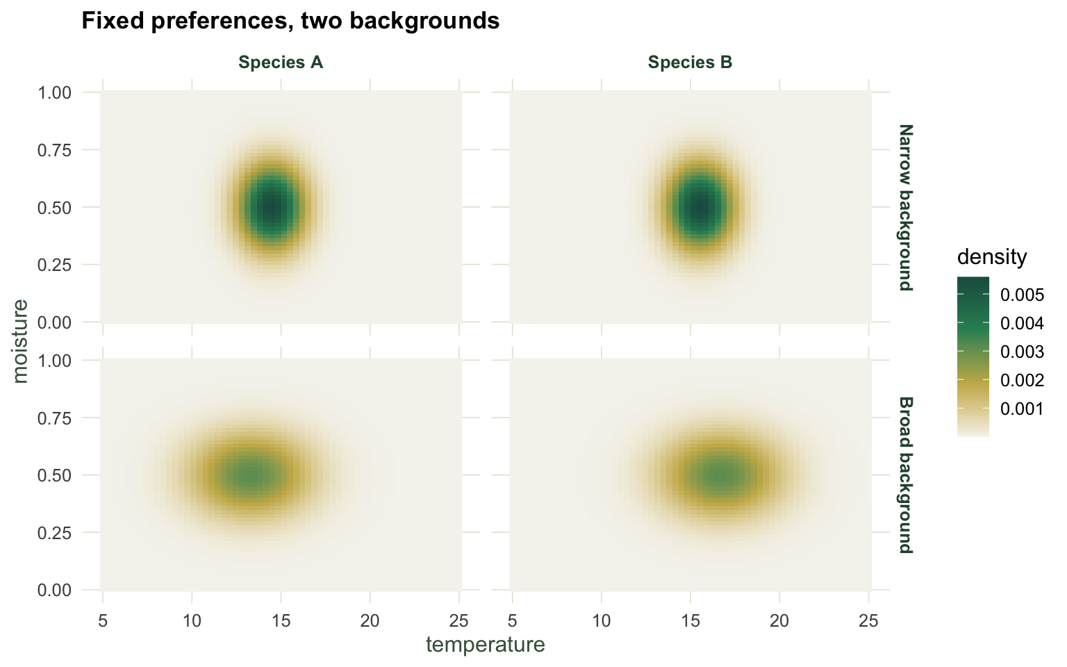
Under the narrow background both species are squeezed toward the middle of the range, where the available climate sits, so their occupied densities pile up in the same place and overlap looks high. Under the broad background each species can occupy the climate it actually prefers, so the two densities pull apart toward 13 and 17. The preferences did not move; the overlap did.
The swing, and the correction that removes it
Sweep the background from narrow to broad and record the raw overlap at each step. Then apply the correction: divide the occupied density by availability to recover the preference, and compute the overlap on those.
sds <- c(1.0, 1.5, 2.5, 4, 6, 10)
D_raw <- D_cor <- numeric(length(sds))
for (i in seq_along(sds)) {
  av <- with(grid, dnorm(temp, 15, sds[i]) * dnorm(moist, 0.5, 0.30)); av <- av / sum(av)
  oA <- occ(prefA, av); oB <- occ(prefB, av)
  D_raw[i] <- schoener_D(oA, oB)
  D_cor[i] <- schoener_D(corrected(oA, av), corrected(oB, av))
}
raw_span <- max(D_raw) - min(D_raw)
cor_span <- max(D_cor) - min(D_cor)
sw <- rbind(
data.frame(sd = sds, D = D_raw, kind = "Raw overlap"),
data.frame(sd = sds, D = D_cor, kind = "Corrected (preference)")
)
ggplot(sw, aes(sd, D, colour = kind)) +
geom_hline(yintercept = D_fund, linetype = "dashed", colour = "#8a8f83") +
geom_line(linewidth = 0.9) + geom_point(size = 2.4) +
scale_x_continuous(transform = "log2", breaks = sds) +
scale_colour_manual(values = c("Raw overlap" = "#b5534e", "Corrected (preference)" = "#275139"), name = NULL) +
scale_y_continuous(limits = c(0.4, 0.8)) +
labs(title = "The background drives the raw overlap",
x = "background breadth (availability SD, log scale)", y = "Schoener's D") +
theme_te() + theme(legend.position = "top")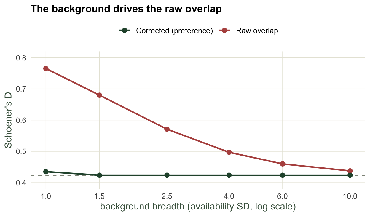
Across these backgrounds the raw overlap runs from 0.765 down to 0.437, a span of 0.328, with the species preferences untouched the whole way. The corrected overlap moves by only 0.011 and stays pinned to the fundamental value of 0.424. The lesson is blunt: a raw overlap number is not comparable across studies with different backgrounds, and two papers reporting different overlaps for the same species pair might differ only in the extent of the region they sampled. If the question is about the species rather than the landscape, the availability-corrected overlap is the one to compare.
The correction is not free
Dividing by availability is the right idea, but it buys less bias with more variance. Where the background is thin and occurrence counts are sparse, the division inflates the density estimate and amplifies sampling noise. Draw finite samples and the cost shows up.
av_b <- with(grid, dnorm(temp, 15, 4) * dnorm(moist, 0.5, 0.30)); av_b <- av_b / sum(av_b)
oA <- occ(prefA, av_b); oB <- occ(prefB, av_b)
St <- { d <- outer(temp, temp, "-"); K <- exp(-0.5 * (d / 2)^2); K / rowSums(K) }
Sm <- { d <- outer(moist, moist, "-"); K <- exp(-0.5 * (d / 0.10)^2); K / rowSums(K) }
ndens <- function(pt, pm) {
  it <- findInterval(pt, c(-Inf, (temp[-1] + temp[-gx]) / 2, Inf))
  im <- findInterval(pm, c(-Inf, (moist[-1] + moist[-gy]) / 2, Inf))
  cnt <- matrix(0, gy, gx); for (k in seq_along(it)) cnt[im[k], it[k]] <- cnt[im[k], it[k]] + 1
  # t() puts the cells back in expand.grid order (temperature varying fastest)
  d <- Sm %*% cnt %*% t(St); as.vector(t(pmax(d, 0))) / sum(d)
}
set.seed(606)
reps <- 200; n <- 100; raw <- cor_ <- numeric(reps)
for (i in 1:reps) {
  ia <- sample.int(nrow(grid), n, replace = TRUE, prob = oA)
  ib <- sample.int(nrow(grid), n, replace = TRUE, prob = oB)
  da <- ndens(grid$temp[ia], grid$moist[ia]); db <- ndens(grid$temp[ib], grid$moist[ib])
  raw[i]  <- schoener_D(da, db)
  cor_[i] <- schoener_D(corrected(da, av_b), corrected(db, av_b))
}
raw_m <- mean(raw); raw_s <- sd(raw); cor_m <- mean(cor_); cor_s <- sd(cor_)
var_amp <- cor_s / raw_s
In 200 replicate samples of 100 occurrences per species under a broad background, the raw overlap averages 0.609 (SD 0.036) and the corrected overlap 0.467 (SD 0.045). The correction pulls the estimate back toward the fundamental value of 0.424, cutting the bias from +0.185 to +0.044, but widens the spread by a factor of 1.3. Two things sit in those numbers. The correction removes the background-breadth part of the bias, not the extra overlap that smoothing a finite sample adds, so the corrected estimate still sits above the fundamental. And the variance it adds is the price of the division: raw overlap is a stable but biased summary, corrected overlap a less biased but noisier one. Here the trade is lopsided, though: the spread the correction adds is small next to the bias it removes, and the corrected estimate lands closer to the fundamental value than the raw one in 200 of the 200 replicates.
What to carry forward
The measured overlap answers a question about occupied environment, which folds together the species and the region. If the comparison is meant to be about the species, correct for availability and accept the variance cost, or at minimum report the background so a raw number can be read in context. The next post gathers this together with the other ways a niche comparison can mislead, and gives a short set of checks to run before trusting one.
Where to go next
The species distribution modelling posts cover fitting the distributions whose overlap this measures, and the resampling posts give the bootstrap machinery for putting uncertainty on a corrected estimate. The final post in this group turns the pitfalls into a checklist.
References
Broennimann, Fitzpatrick, Pearman, Petitpierre, Pellissier, Yoccoz, Thuiller, Fortin, Randin, Zimmermann, Graham, Guisan 2012 Global Ecology and Biogeography 21(4):481-497 (10.1111/j.1466-8238.2011.00698.x)
Warren, Glor, Turelli 2008 Evolution 62(11):2868-2883 (10.1111/j.1558-5646.2008.00482.x)
Soberon 2007 Ecology Letters 10(12):1115-1123 (10.1111/j.1461-0248.2007.01107.x)
Colwell, Rangel 2009 Proceedings of the National Academy of Sciences 106(Suppl 2):19651-19658 (10.1073/pnas.0901650106)