library(ggplot2)

theme_te <- function() {
  theme_minimal(base_size = 12) +
    theme(
          plot.background  = element_rect(fill = "#f5f4ee", colour = NA),
          panel.background = element_rect(fill = "#f5f4ee", colour = NA),
          panel.grid.minor = element_blank(),
      panel.grid.major = element_line(colour = "#e7e6da", linewidth = 0.3),
      plot.title = element_text(face = "bold", size = 13),
      axis.title = element_text(colour = "#46604a"),
      strip.text = element_text(face = "bold", colour = "#275139")
    )
}Niche equivalency and similarity tests
R
niche overlap
hypothesis testing
species distribution models
ecology tutorial
Permutation tests for niche overlap in R: the equivalency test asks if two species share a niche, the similarity test whether they are more alike than chance.
Corrected 7 October 2026: the post said that the background similarity test sidesteps the equivalency test’s problem at large sample sizes by asking a graded question; it now says that the similarity test asks a directional question but also tests a point null, so it too rejects small departures once samples are large, and that at large samples it is judged by the gap between the observed overlap and its null rather than by the p-value alone.
A raw overlap value on its own says nothing. Two species can share a Schoener’s D of 0.55, but whether that counts as similar or different depends on what you compare it against. The two standard permutation tests, introduced with ENMTools, each supply a different comparison, and they answer genuinely different questions. This post builds both from occurrence points, checks that the first one is calibrated, and then shows the limit that catches people out: the equivalency test rejects a shared niche for essentially any pair of real species once the sample is large enough, so a rejection is not evidence of ecological difference. The background similarity test asks a different, directional question, whether the two species are more or less alike than the available environment would make them, but it does not sidestep the problem: it also tests a point null, so it too rejects small departures once the sample is large.
If you have not met Schoener’s D and Warren’s I yet, the previous post builds them from scratch.
Two tests, two null hypotheses
The equivalency test asks whether two species occupy one and the same niche. Pool the occurrences of both species, reshuffle the pooled points into two groups of the original sizes, and recompute the overlap. Repeat many times to build a null distribution of overlaps you would see if the two samples came from a single niche. If the observed overlap sits well below that null, the shared-niche hypothesis is rejected.
The background similarity test asks a softer question: is the observed overlap more (or less) than you would expect if one species were scattered at random across the available environment? Hold one species fixed, replace the other with random draws from the background, recompute the overlap, and repeat. Observed overlap above the null means the two are more alike than chance (niche conservatism); below the null means more different than chance (niche divergence).
The environmental space is a temperature by moisture grid. A niche density is built by binning occurrence points to the grid, smoothing with a separable Gaussian kernel, and normalising to sum to one. That is a fast, transparent stand-in for a fitted distribution, and it keeps the permutation loops cheap enough to run thousands of times.
gx <- 40; gy <- 40
temp  <- seq(5, 25, length.out = gx)
moist <- seq(0, 1, length.out = gy)
grid  <- expand.grid(temp = temp, moist = moist)

smoother <- function(ax, bw) {
  K <- exp(-0.5 * (outer(ax, ax, "-") / bw)^2)
  K / rowSums(K)
}
St <- smoother(temp, 2.0); Sm <- smoother(moist, 0.10)

niche_density <- function(pt, pm) {
  it <- findInterval(pt, c(-Inf, (temp[-1] + temp[-gx]) / 2, Inf))
  im <- findInterval(pm, c(-Inf, (moist[-1] + moist[-gy]) / 2, Inf))
  cnt <- matrix(0, gy, gx)
  for (k in seq_along(it)) cnt[im[k], it[k]] <- cnt[im[k], it[k]] + 1
  d <- Sm %*% cnt %*% t(St)
  as.vector(pmax(d, 0)) / sum(d)
}
schoener_D <- function(p, q) sum(pmin(p, q))

avail <- with(grid, dnorm(temp, 15, 4) * dnorm(moist, 0.5, 0.22))
avail <- avail / sum(avail)
draw_occ <- function(n, t0, m0, st = 2.5, sm = 0.14) {
  w <- avail * with(grid, dnorm(grid$temp, t0, st) * dnorm(grid$moist, m0, sm))
  idx <- sample.int(nrow(grid), n, replace = TRUE, prob = w)
  list(t = grid$temp[idx], m = grid$moist[idx])
}
draw_bg <- function(n) {
  idx <- sample.int(nrow(grid), n, replace = TRUE, prob = avail)
  list(t = grid$temp[idx], m = grid$moist[idx])
}

equiv_test <- function(oa, ob, R = 199) {
  nA <- length(oa$t); nB <- length(ob$t)
  allt <- c(oa$t, ob$t); allm <- c(oa$m, ob$m)
  Dobs <- schoener_D(niche_density(oa$t, oa$m), niche_density(ob$t, ob$m))
  Dnull <- numeric(R)
  for (r in 1:R) {
    s <- sample.int(nA + nB); ga <- s[1:nA]; gb <- s[(nA + 1):(nA + nB)]
    Dnull[r] <- schoener_D(niche_density(allt[ga], allm[ga]),
                           niche_density(allt[gb], allm[gb]))
  }
  list(Dobs = Dobs, p = (sum(Dnull <= Dobs) + 1) / (R + 1), Dnull = Dnull)
}
sim_test <- function(oa, ob, R = 199) {
  pa <- niche_density(oa$t, oa$m)
  Dobs <- schoener_D(pa, niche_density(ob$t, ob$m))
  nB <- length(ob$t); Dnull <- numeric(R)
  for (r in 1:R) { bg <- draw_bg(nB); Dnull[r] <- schoener_D(pa, niche_density(bg$t, bg$m)) }
  list(Dobs = Dobs, Dnull = Dnull,
       p_more = (sum(Dnull >= Dobs) + 1) / (R + 1),
       p_less = (sum(Dnull <= Dobs) + 1) / (R + 1))
}
The equivalency test is calibrated
Before trusting a test, check that it rejects at the stated rate when the null is true. Draw both species from the same niche (identical preference centre), run the equivalency test, and count how often it rejects at the 5% level. Over many replicates the rejection rate should land near 0.05.
set.seed(101)
reps <- 200; rej_same <- logical(reps)
for (i in 1:reps) {
  oa <- draw_occ(80, 15, 0.5); ob <- draw_occ(80, 15, 0.5)   # one shared niche
  rej_same[i] <- equiv_test(oa, ob, R = 99)$p < 0.05
}
rej_rate <- mean(rej_same)
When both species genuinely share a niche, the equivalency test rejects in 5.5% of replicates, close to the nominal 5%. The test controls its error rate: that is exactly what makes the next result a problem rather than a bug.
The limit: a fixed tiny difference becomes certain rejection
Now fix a small, constant difference between the two niches (their preference centres sit 1.5 temperature units apart, well under one standard deviation) and hold it there while the sample size grows. The difference never changes. Only n does.
set.seed(202)
ns <- c(30, 60, 120, 240, 480); reps2 <- 150; off <- 1.5
rej_n <- numeric(length(ns))
for (j in seq_along(ns)) {
  rj <- logical(reps2)
  for (i in 1:reps2) {
    oa <- draw_occ(ns[j], 15 - off/2, 0.5)
    ob <- draw_occ(ns[j], 15 + off/2, 0.5)
    rj[i] <- equiv_test(oa, ob, R = 99)$p < 0.05
  }
  rej_n[j] <- mean(rj)
}
mag <- data.frame(n = ns, rejection = rej_n)ggplot(mag, aes(n, rejection)) +
geom_hline(yintercept = 0.05, linetype = "dashed", colour = "#b5534e") +
geom_line(colour = "#275139", linewidth = 0.9) +
geom_point(colour = "#275139", size = 2.6) +
scale_x_continuous(transform = "log2", breaks = ns) +
scale_y_continuous(limits = c(0, 1)) +
annotate("text", x = 30, y = 0.10, label = "nominal 5%",
hjust = 0, size = 3.3, colour = "#b5534e") +
labs(title = "A fixed niche difference always rejects, given enough data",
x = "sample size per species (log scale)", y = "rejection rate") +
theme_te()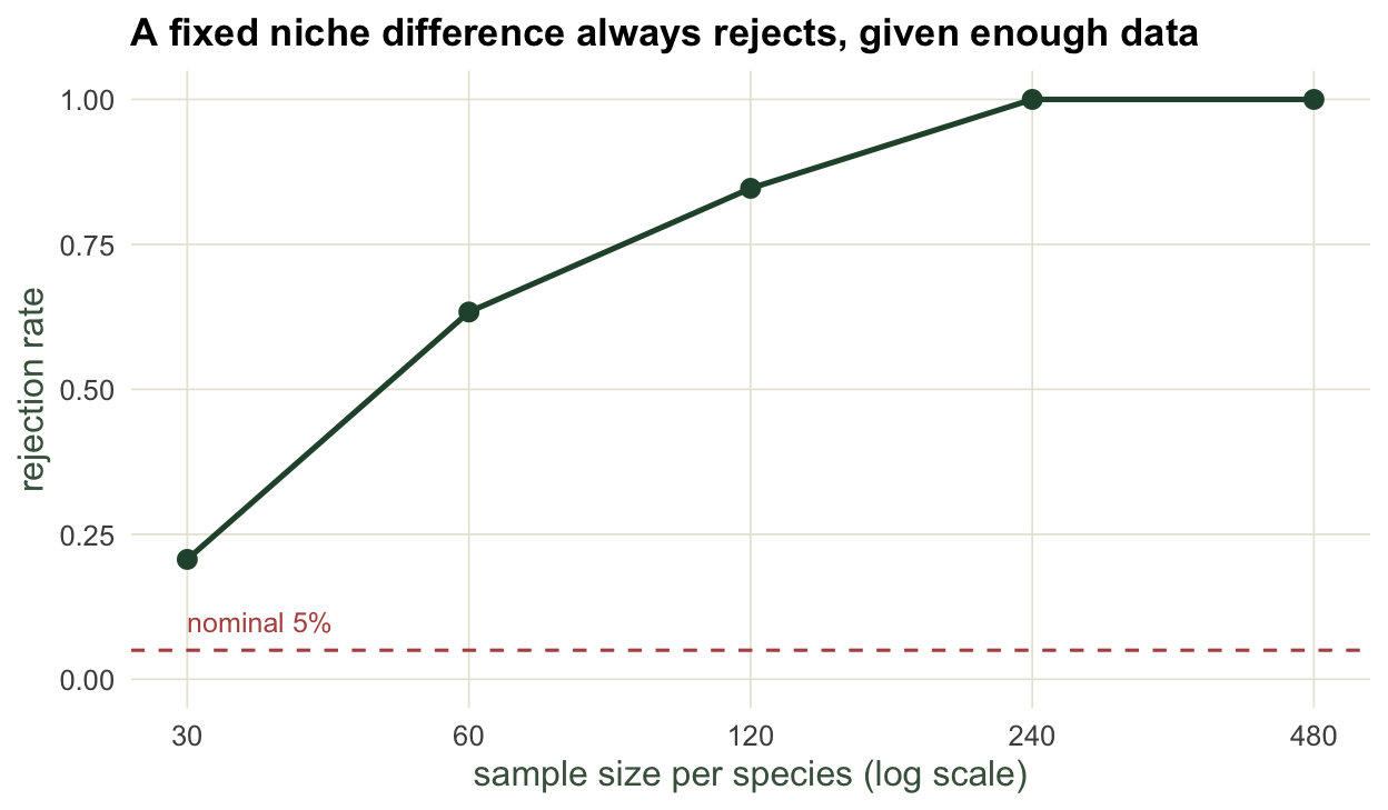
The rejection rate runs 0.21, 0.63, 0.85, 1.00, 1.00 across n = 30, 60, 120, 240, 480. The niches never changed. What changed is the test’s power to detect a difference that was there all along. This is the general behaviour of a point-null hypothesis: perfect equivalence is a knife-edge that no two real species sit on, so a large enough sample rejects it every time. A significant equivalency test at n = 500 tells you the two niches are not byte-identical. It does not tell you they are ecologically different, and it certainly does not measure how different.
The similarity test separates what the equivalency test cannot
Take two contrasting pairs. The first is two moderately similar species (preference centres 14 and 16); the second is a divergent pair (centres 11 and 20). Run the equivalency test on both, then the background similarity test on both.
set.seed(303)
oa <- draw_occ(200, 14, 0.48); ob <- draw_occ(200, 16, 0.52)
eq1 <- equiv_test(oa, ob, R = 299)
si1 <- sim_test(oa, ob, R = 299)set.seed(404)
oc <- draw_occ(200, 11, 0.35); od <- draw_occ(200, 20, 0.70)
eq2 <- equiv_test(oc, od, R = 299)
si2 <- sim_test(oc, od, R = 299)The equivalency test rejects a shared niche for both pairs at the same p-value, 0.0033, which is the smallest value reachable with 299 permutations. The similar pair has observed D = 0.769; the divergent pair D = 0.174. Those overlaps could hardly be more different, yet the equivalency test returns an identical verdict, because both pairs fail the point-null of exact identity and it has no scale beyond pass or fail.
The similarity test separates them. For the similar pair, observed overlap (0.769) sits above the random-background null (mean 0.704), with p for more-similar-than-chance equal to 0.0033: the two species are more alike than a random pick from the available environment, the signature of niche conservatism. For the divergent pair, observed overlap (0.174) falls below its null (mean 0.552), with p for more-different-than-chance equal to 0.0033: more different than chance, the signature of niche divergence.
sc <- rbind(
  data.frame(D = si1$Dnull, pair = "Similar pair (14 vs 16)", obs = si1$Dobs),
  data.frame(D = si2$Dnull, pair = "Divergent pair (11 vs 20)", obs = si2$Dobs)
)
sc$pair <- factor(sc$pair, levels = c("Similar pair (14 vs 16)", "Divergent pair (11 vs 20)"))
obs_df <- unique(sc[, c("pair", "obs")])
ggplot(sc, aes(D)) +
  geom_histogram(bins = 30, fill = "#93a87f", colour = "white", linewidth = 0.15) +
  geom_vline(data = obs_df, aes(xintercept = obs), colour = "#b5534e", linewidth = 0.9) +
  facet_wrap(~pair, scales = "free_x") +
  labs(title = "Same equivalency verdict, opposite similarity verdict",
       x = "Schoener's D", y = "count") +
  theme_te()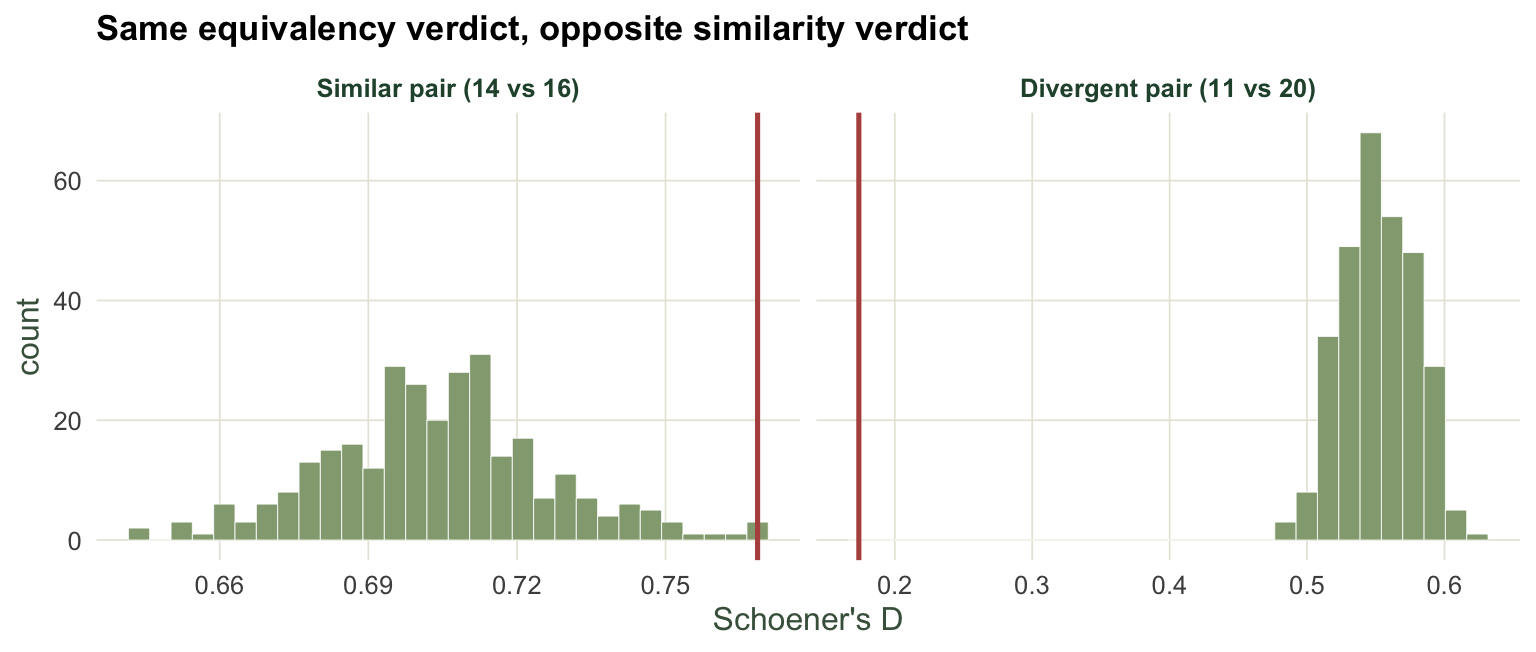
Which test answers your question
The two tests are not competitors; they answer different questions and the equivalency test is the narrower of the two. Use the equivalency test when the hypothesis really is strict identity, and read a rejection as no more than that: not one shared niche. Do not read it as a measure of ecological difference, and be wary of it at large sample sizes, where it rejects almost everything. Use the background similarity test when the question is comparative, whether two species are more alike, or more different, than the environment they had available would produce by chance. That comparative answer is usually the one the ecology actually needs, but the similarity test also tests a point null, so at large sample sizes judge it by the gap between the observed overlap and its null, not by the p-value alone.
One asymmetry is lurking in the similarity test: holding species A fixed and randomising B need not give the same verdict as the reverse, because the null distribution depends on which density is held fixed while the other species is redrawn from the background. That direction-dependence, and the wider problem of the background quietly driving the result, is the subject of the next post.
Where to go next
The next post shows how the measured overlap moves with the environmental background even when the species’ preferences are fixed, and how to correct for it. For the general logic of permutation and randomisation tests, the resampling posts give the foundations that this niche-specific version rests on.
References
Warren, Glor, Turelli 2008 Evolution 62(11):2868-2883 (10.1111/j.1558-5646.2008.00482.x)
Warren, Glor, Turelli 2010 Ecography 33(3):607-611 (10.1111/j.1600-0587.2009.06142.x)
Peterson, Soberon, Sanchez-Cordero 1999 Science 285(5431):1265-1267 (10.1126/science.285.5431.1265)
Broennimann, Fitzpatrick, Pearman, Petitpierre, Pellissier, Yoccoz, Thuiller, Fortin, Randin, Zimmermann, Graham, Guisan 2012 Global Ecology and Biogeography 21(4):481-497 (10.1111/j.1466-8238.2011.00698.x)