library(ggplot2)

theme_te <- function() {
  theme_minimal(base_size = 12) +
    theme(
          plot.background  = element_rect(fill = "#f5f4ee", colour = NA),
          panel.background = element_rect(fill = "#f5f4ee", colour = NA),
          panel.grid.minor = element_blank(),
      panel.grid.major = element_line(colour = "#e7e6da", linewidth = 0.3),
      plot.title = element_text(face = "bold", size = 13),
      axis.title = element_text(colour = "#46604a"),
      strip.text = element_text(face = "bold", colour = "#275139")
    )
}
paper_forest <- c("#f5f4ee", "#c9b458", "#2f8f63", "#1d5b4e")

gx <- 50; gy <- 50
temp  <- seq(5, 25, length.out = gx)
moist <- seq(0, 1, length.out = gy)
grid  <- expand.grid(temp = temp, moist = moist)
schoener_D <- function(p, q) sum(pmin(p, q))
avail <- with(grid, dnorm(temp, 15, 4) * dnorm(moist, 0.5, 0.22)); avail <- avail / sum(avail)Checking a niche comparison
R
niche overlap
model checking
species distribution models
ecology tutorial
A checklist for niche overlap analyses in R: bandwidth sensitivity, realised versus fundamental niches, and the direction-dependence of the similarity test.
Corrected 1 October 2026: check three compared an observed overlap between the two exact niches with null draws built from smoothed samples; both niches are now estimated from smoothed occurrence samples, as the null draws are, and against the narrow background the observed overlap now sits inside the null rather than at its low edge, while the two directions still disagree.
A niche overlap number can be wrong in ways that never announce themselves. The code runs, a value between 0 and 1 comes out, a permutation test attaches a p-value, and nothing flags that the result is an artefact of a smoothing choice, a truncated range, or the direction the test happened to run. This closing post in the niche-overlap group collects three checks worth running before a comparison is trusted. Each is a short piece of code, and each targets a failure that looks exactly like a real signal.
The earlier posts in the group build the tools: Schoener’s D and Warren’s I, the permutation tests, and the background dependence of the raw number.
Check 1: the smoothing bandwidth moves the answer more than sampling does
A kernel-smoothed overlap has a free parameter, the bandwidth, and it is rarely reported. Widen the smoothing and the two density blobs spread and overlap more; narrow it and they sharpen and overlap less. On one fixed dataset the estimate can travel across nearly a third of the 0 to 1 scale as the bandwidth alone changes.
prefA <- with(grid, dnorm(temp, 14, 2.5) * dnorm(moist, 0.5, 0.14))
prefB <- with(grid, dnorm(temp, 17, 2.5) * dnorm(moist, 0.5, 0.14))
oA <- prefA * avail; oA <- oA / sum(oA)
oB <- prefB * avail; oB <- oB / sum(oB)

mk_smoother <- function(bt, bm) {
  St <- { d <- outer(temp, temp, "-"); K <- exp(-0.5 * (d / bt)^2); K / rowSums(K) }
  Sm <- { d <- outer(moist, moist, "-"); K <- exp(-0.5 * (d / bm)^2); K / rowSums(K) }
  list(St = St, Sm = Sm)
}
ndens <- function(pt, pm, S) {
  it <- findInterval(pt, c(-Inf, (temp[-1] + temp[-gx]) / 2, Inf))
  im <- findInterval(pm, c(-Inf, (moist[-1] + moist[-gy]) / 2, Inf))
  cnt <- matrix(0, gy, gx); for (k in seq_along(it)) cnt[im[k], it[k]] <- cnt[im[k], it[k]] + 1
  # t() before as.vector(): expand.grid varies temp fastest, as.vector() is column-major
  d <- S$Sm %*% cnt %*% t(S$St); as.vector(t(pmax(d, 0))) / sum(d)
}

set.seed(909); n <- 120
ia <- sample.int(nrow(grid), n, replace = TRUE, prob = oA)
ib <- sample.int(nrow(grid), n, replace = TRUE, prob = oB)
ta <- grid$temp[ia]; ma <- grid$moist[ia]
tb <- grid$temp[ib]; mb <- grid$moist[ib]
bws <- c(0.8, 1.5, 2.5, 4, 6)
Dbw <- numeric(length(bws))
for (j in seq_along(bws)) {
S <- mk_smoother(bws[j], bws[j] * 0.05)
Dbw[j] <- schoener_D(ndens(ta, ma, S), ndens(tb, mb, S))
}
bw_range <- max(Dbw) - min(Dbw)
# bootstrap CI at a single fixed bandwidth: the sampling uncertainty
S0 <- mk_smoother(2.5, 0.12)
Dhat <- schoener_D(ndens(ta, ma, S0), ndens(tb, mb, S0))
B <- 400; Db <- numeric(B)
for (b in 1:B) {
ra <- sample.int(n, n, replace = TRUE); rb <- sample.int(n, n, replace = TRUE)
Db[b] <- schoener_D(ndens(ta[ra], ma[ra], S0), ndens(tb[rb], mb[rb], S0))
}
ci <- quantile(Db, c(0.025, 0.975))
ci_width <- unname(ci[2] - ci[1])
dominance <- bw_range / ci_widthdfb <- data.frame(bw = bws, D = Dbw)
ggplot(dfb, aes(bw, D)) +
geom_line(colour = "#275139", linewidth = 0.9) +
geom_point(colour = "#275139", size = 2.6) +
annotate("errorbar", x = 2.5, ymin = ci[1], ymax = ci[2],
width = 0.25, colour = "#b5534e", linewidth = 0.8) +
annotate("text", x = 2.75, y = Dhat, hjust = 0, size = 3.2, colour = "#b5534e",
label = "bootstrap 95% CI\n(sampling)") +
labs(title = "Bandwidth moves D more than sampling does",
x = "smoothing bandwidth (temperature)", y = "Schoener's D") +
theme_te()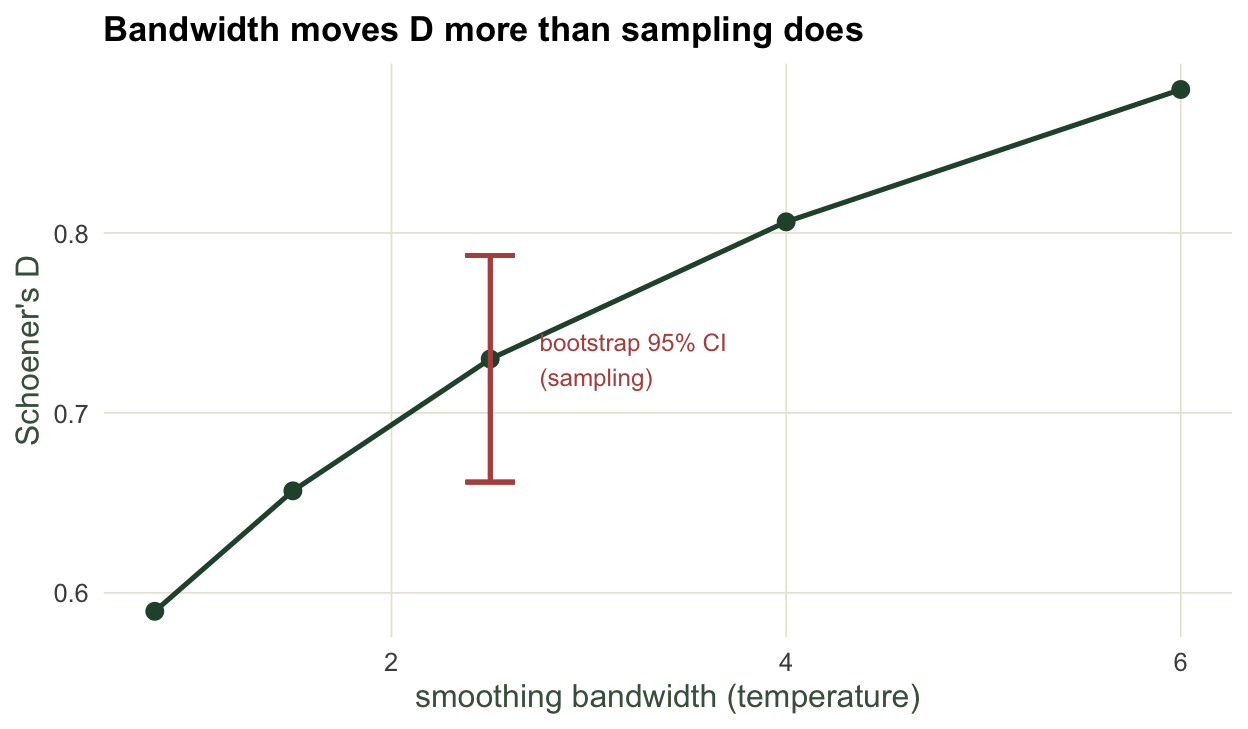
On this single dataset the estimate ranges from 0.590 to 0.880 as the bandwidth alone changes, a span of 0.290. The point estimate at a fixed bandwidth of 2.5 is 0.730, with a bootstrap 95% interval of [0.662, 0.788], a width of 0.126. The tuning choice moves the answer 2.3 times as far as sampling error, so a bare D with no bandwidth reported is barely interpretable. Report the bandwidth, fix it by a rule rather than by eye, and put a bootstrap interval on the estimate so the sampling uncertainty is visible next to it.
Check 2: a low overlap can be geography, not biology
Two species can have the exact same environmental preference and still show almost no overlap, if they never had access to the same environments. Give both an identical fundamental niche centred at 15 degrees, then let one occupy only the cold half of the range and the other only the warm half. Nothing about their biology differs. The measured overlap collapses anyway.
pref <- with(grid, dnorm(temp, 15, 3) * dnorm(moist, 0.5, 0.16)); pref <- pref / sum(pref)
D_fund <- schoener_D(pref, pref)                       # identical preference: overlap is 1
av_cold <- with(grid, ifelse(temp < 15, 1, 0.03)) * avail; av_cold <- av_cold / sum(av_cold)
av_warm <- with(grid, ifelse(temp > 15, 1, 0.03)) * avail; av_warm <- av_warm / sum(av_warm)
occA <- pref * av_cold; occA <- occA / sum(occA)
occB <- pref * av_warm; occB <- occB / sum(occB)
D_real <- schoener_D(occA, occB)
gap <- D_fund - D_real
dft <- rbind(
data.frame(grid, dens = occA, species = "Species A (cold access)"),
data.frame(grid, dens = occB, species = "Species B (warm access)")
)
ggplot(dft, aes(temp, moist, fill = dens)) +
geom_raster() +
facet_wrap(~species) +
scale_fill_gradientn(colours = paper_forest, name = "density") +
labs(title = "Same preference, non-overlapping realised niches",
x = "temperature", y = "moisture") +
theme_te()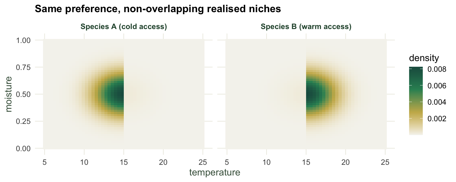
The fundamental-niche overlap is D = 1.000, since the two preferences are identical. The realised overlap is D = 0.058, a truncation gap of 0.942. A reader handed only the realised number would conclude the two species have sharply different niches, when the difference is entirely in where they can live, not what they tolerate. Before reading a low overlap as ecological divergence, check whether the two species even sampled overlapping environments; if their accessible ranges barely meet, the overlap is measuring geography.
Check 3: the similarity test can disagree with itself
The background similarity test holds one species fixed and randomises the other against its background. When the two species have different backgrounds, the test is directional: running it one way can give the opposite verdict to running it the other way. Here species A has a broad accessible range and B a narrow one. Each species’ niche is estimated from an occurrence sample of the same size as the null samples and smoothed with the same kernel, so the observed overlap and the null draws are the same statistic.
prefX <- with(grid, dnorm(temp, 15,   2.5) * dnorm(moist, 0.5, 0.14))
prefY <- with(grid, dnorm(temp, 16.5, 2.5) * dnorm(moist, 0.5, 0.14))
avBroad  <- with(grid, dnorm(temp, 15, 7.0) * dnorm(moist, 0.5, 0.35)); avBroad  <- avBroad  / sum(avBroad)
avNarrow <- with(grid, dnorm(temp, 16, 2.2) * dnorm(moist, 0.5, 0.16)); avNarrow <- avNarrow / sum(avNarrow)
oX <- prefX * avBroad;  oX <- oX / sum(oX)
oY <- prefY * avNarrow; oY <- oY / sum(oY)

St2 <- { d <- outer(temp, temp, "-"); K <- exp(-0.5 * (d / 2)^2); K / rowSums(K) }
Sm2 <- { d <- outer(moist, moist, "-"); K <- exp(-0.5 * (d / 0.10)^2); K / rowSums(K) }
nd2 <- function(pt, pm) {
  it <- findInterval(pt, c(-Inf, (temp[-1] + temp[-gx]) / 2, Inf))
  im <- findInterval(pm, c(-Inf, (moist[-1] + moist[-gy]) / 2, Inf))
  cnt <- matrix(0, gy, gx); for (k in seq_along(it)) cnt[im[k], it[k]] <- cnt[im[k], it[k]] + 1
  d <- Sm2 %*% cnt %*% t(St2); as.vector(t(pmax(d, 0))) / sum(d)   # grid order, as above
}
set.seed(808)
# both niches estimated from 300 occurrences, smoothed like the null samples
idxX <- sample.int(nrow(grid), 300, replace = TRUE, prob = oX)
idxY <- sample.int(nrow(grid), 300, replace = TRUE, prob = oY)
eX <- nd2(grid$temp[idxX], grid$moist[idxX]); eY <- nd2(grid$temp[idxY], grid$moist[idxY])
D_obs <- schoener_D(eX, eY); R <- 499
# A -> B: hold X, draw the null from B's narrow background
dnA <- numeric(R)
for (r in 1:R) { idx <- sample.int(nrow(grid), 300, replace = TRUE, prob = avNarrow); dnA[r] <- schoener_D(eX, nd2(grid$temp[idx], grid$moist[idx])) }
# B -> A: hold Y, draw the null from A's broad background
dnB <- numeric(R)
for (r in 1:R) { idx <- sample.int(nrow(grid), 300, replace = TRUE, prob = avBroad); dnB[r] <- schoener_D(eY, nd2(grid$temp[idx], grid$moist[idx])) }
pA_more <- (sum(dnA >= D_obs) + 1) / (R + 1)
pB_more <- (sum(dnB >= D_obs) + 1) / (R + 1)
asym <- rbind(
data.frame(D = dnA, dir = "A held, null from B (narrow)", obs = D_obs),
data.frame(D = dnB, dir = "B held, null from A (broad)", obs = D_obs)
)
asym$dir <- factor(asym$dir, levels = c("A held, null from B (narrow)", "B held, null from A (broad)"))
obs_df <- unique(asym[, c("dir", "obs")])
ggplot(asym, aes(D)) +
geom_histogram(bins = 30, fill = "#93a87f", colour = "white", linewidth = 0.15) +
geom_vline(data = obs_df, aes(xintercept = obs), colour = "#b5534e", linewidth = 0.9) +
facet_wrap(~dir, scales = "free_x") +
labs(title = "Same pair, opposite similarity verdict",
x = "Schoener's D", y = "count") +
theme_te() +
theme(panel.spacing.x = unit(2, "lines"),
panel.border = element_rect(colour = "grey70", fill = NA))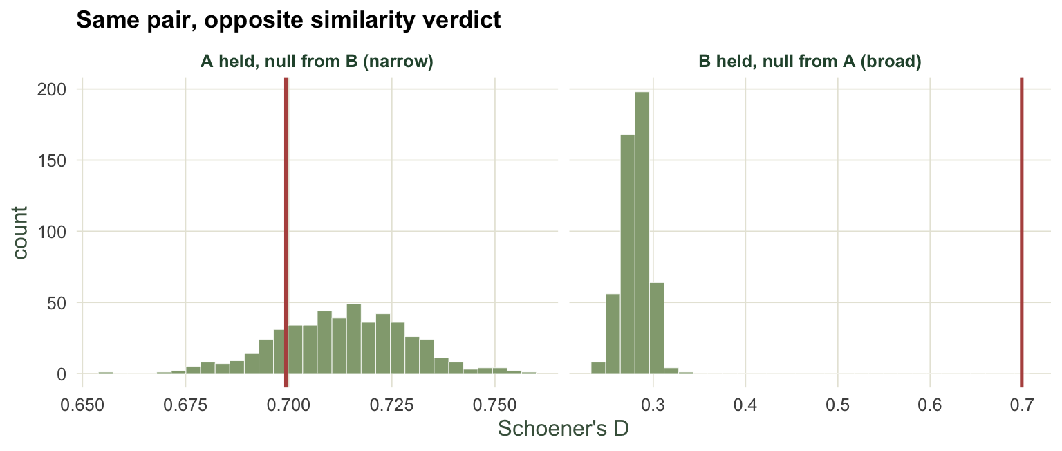
The observed overlap is D = 0.818 in both directions. Holding A and drawing the null from B’s narrow background, the observed overlap sits inside the null, whose mean is 0.823, with p for more-similar-than-chance equal to 0.584: no evidence that the two are more alike than B’s background alone would produce. Holding B and drawing the null from A’s broad background, the null mean drops to 0.468 and the same observed overlap is now far above it, with p = 0.0020: strong evidence of similarity. Same species, same overlap, opposite conclusions, purely because the two backgrounds differ. Run the similarity test in both directions and report both; if they disagree, the disagreement is the finding, and a single-direction test would have hidden it.
The checklist
Before trusting a niche comparison, run through four questions. Is the smoothing bandwidth reported and fixed by a rule, with a bootstrap interval on the estimate? Do the two species have overlapping accessible environments, so a low overlap cannot be pure range truncation? Has the similarity test been run in both directions, with both reported? And is the overlap corrected for availability, or at least reported alongside the background so it can be read in context? That last question is worked through in the background dependence post rather than here. None of these needs heavy machinery. Each takes a few lines, and each catches a way that a clean-looking number can be quietly meaningless.
Where to go next
The species distribution modelling posts cover fitting the underlying distributions, the resampling posts give the bootstrap and permutation foundations these checks lean on, and the model-checking posts extend the same habit of interrogating a result to regression and ordination. That closes the niche-overlap group.
References
Warren, Glor, Turelli 2008 Evolution 62(11):2868-2883 (10.1111/j.1558-5646.2008.00482.x)
Warren, Glor, Turelli 2010 Ecography 33(3):607-611 (10.1111/j.1600-0587.2009.06142.x)
Guisan, Petitpierre, Broennimann, Daehler, Kueffer 2014 Trends in Ecology and Evolution 29(5):260-269 (10.1016/j.tree.2014.02.009)
Soberon 2007 Ecology Letters 10(12):1115-1123 (10.1111/j.1461-0248.2007.01107.x)