library(vegan)
library(ggplot2)

theme_te <- function(base_size = 12) {
  theme_minimal(base_size = base_size) +
    theme(
      plot.background  = element_rect(fill = "#f5f4ee", colour = NA),
      panel.background = element_rect(fill = "#f5f4ee", colour = NA),
      panel.grid.major = element_line(colour = "#dad9ca", linewidth = 0.3),
      panel.grid.minor = element_blank(),
      axis.text   = element_text(colour = "#46604a"),
      axis.title  = element_text(colour = "#2c3a31"),
      plot.title  = element_text(colour = "#16241d", face = "bold"),
      plot.subtitle = element_text(colour = "#5d6b61"),
      strip.text  = element_text(colour = "#16241d", face = "bold"),
      legend.position = "none"
    )
}
forest <- "#275139"; red <- "#b5534e"; faint <- "#5d6b61"
paper  <- "#f5f4ee"; line <- "#dad9ca"

tile_df <- function(M, label) {
  d <- as.data.frame(as.table(M))
  names(d) <- c("site", "species", "pa")
  d$site    <- as.integer(d$site)
  d$species <- as.integer(d$species)
  d$pa      <- factor(d$pa, levels = c(0, 1))
  d$panel   <- label
  d
}
mat_theme <- theme_te() +
  theme(panel.grid = element_blank(), axis.text = element_blank(),
axis.ticks = element_blank())Nestedness, NODF, and null models in R
ecology tutorial
R
vegan
nestedness
null models
community ecology
beta diversity
Measure community nestedness with the NODF metric in R using vegan, then test it with fixed-margin null models and see why the null choice decides the verdict.
Some communities are nested: the species found at poor sites are a tidy subset of those found at rich sites, so a species-poor island holds nothing you would not also find on a richer one. Nestedness is one of the oldest descriptions of community structure, and the NODF metric of Almeida-Neto and colleagues (2008) turned it into a single number between 0 and 100. Computing that number in R takes one line. Deciding whether it means anything takes a null model, and the null model you pick can flip the answer completely.
This post builds a nested community, measures it with NODF using vegan, and then tests it against two different null models that reach opposite verdicts on the same matrix. The gap between them is the whole lesson.
Nestedness versus turnover
Nestedness is a claim about subsets, not about species replacement. It is worth separating from its opposite, turnover, before measuring anything. Under turnover, poor sites do not hold subsets of rich sites; they hold different species altogether, as happens along a strong environmental gradient where each species occupies its own stretch.
ns <- 20; np <- 30
Rn <- round(seq(np * 0.92, np * 0.12, length.out = ns))
Mn <- matrix(0, ns, np); for (i in seq_len(ns)) Mn[i, seq_len(Rn[i])] <- 1
Mt <- matrix(0, ns, np); bw <- 4
for (j in seq_len(np)) {
  c0 <- (j - 1) / (np - 1) * (ns - 1) + 1
  rr <- round(c0) + (-bw:bw); rr <- rr[rr >= 1 & rr <= ns]
  Mt[rr, j] <- 1
}
d_concept <- rbind(tile_df(Mn, "nested: poorer sites hold subsets"),
                   tile_df(Mt, "turnover: sites hold different species"))

ggplot(d_concept, aes(species, site, fill = pa)) +
  geom_tile(colour = paper, linewidth = 0.25) +
  facet_wrap(~panel) +
  scale_fill_manual(values = c("0" = line, "1" = forest)) +
  scale_y_reverse() + coord_equal() +
  labs(x = "species (ordered by prevalence)", y = "site (ordered by richness)",
       title = "Two ways a community can be structured",
       subtitle = "nestedness is subset structure, not species replacement") +
  mat_theme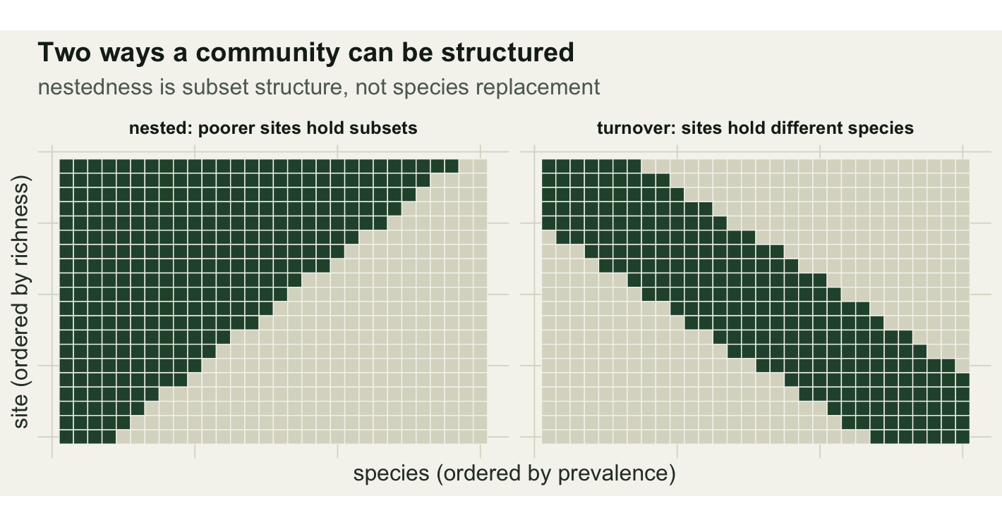
NODF measures how close a real community sits to the left-hand picture. A checkerboard or a band scores low; a clean triangle scores high.
Measuring nestedness with NODF
We simulate a community where each species has a prevalence and each site a richness, both drawn from smooth gradients, so common species turn up almost everywhere and rich sites hold almost everything. That combination produces nestedness.
set.seed(41)
n_site <- 25; n_sp <- 50
site_q <- seq(2.6, -2.6, length.out = n_site)   # site suitability, rich to poor
sp_c   <- seq(2.6, -2.6, length.out = n_sp)     # species commonness, common to rare
P      <- outer(site_q, sp_c, function(a, b) plogis(a + b))
comm   <- matrix(rbinom(n_site * n_sp, 1, P), n_site, n_sp)
comm   <- comm[rowSums(comm) > 0, colSums(comm) > 0]
dim(comm)
[1] 25 50NODF works on the sorted incidence matrix. It rewards two things: fill that decreases from richer to poorer rows and from commoner to rarer columns, and paired overlap, where the occupied cells of a poorer row fall inside those of a richer one. The row score, the column score, and their combination all run from 0 to 100.
nd <- nestednodf(comm)
nodf_val <- nd$statistic[["NODF"]]
round(c(N.columns = nd$statistic[["N.columns"]],
        N.rows    = nd$statistic[["N.rows"]],
        NODF      = nd$statistic[["NODF"]]), 1)
N.columns N.rows NODF
81.1 80.6 81.0 The community scores 81. Sorting rows and columns by their totals makes the pattern visible: the presences pack towards the upper-left, with rich sites and common species crowded together and a thinning tail of rare species and poor sites.
ro <- order(rowSums(comm), decreasing = TRUE)
co <- order(colSums(comm), decreasing = TRUE)
d_mat <- tile_df(comm[ro, co], "sorted")

ggplot(d_mat, aes(species, site, fill = pa)) +
  geom_tile(colour = paper, linewidth = 0.15) +
  scale_fill_manual(values = c("0" = line, "1" = forest)) +
  scale_y_reverse() + coord_equal() +
  labs(x = "species (common to rare)", y = "site (rich to poor)",
       title = paste0("A simulated community with NODF = ", sprintf("%.0f", nodf_val)),
       subtitle = "rows and columns sorted by total: presence packs to the upper left") +
  mat_theme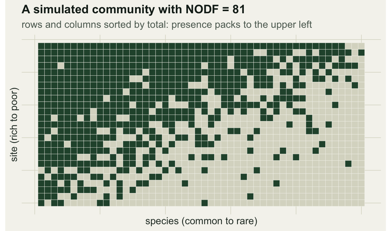
Is 81 a lot? The null model decides
A raw NODF value has no meaning on its own, because even random data with uneven richness and prevalence will score above zero. To judge it, compare the observed value against matrices generated under a null model that keeps some features of the data and randomises the rest. oecosimu does exactly this: it shuffles the matrix many times, recomputes NODF each time, and reports where the observed value falls.
Everything hinges on what the null model holds fixed. The simplest null, r00, keeps only the total number of occurrences and scatters them at random, so row and column totals are free to vary. A stricter null, quasiswap, holds every row total and every column total exactly as observed and randomises only the arrangement of cells within those constraints.
set.seed(7)
os_ff <- oecosimu(comm, nestednodf, method = "quasiswap",
                  nsimul = 999, alternative = "greater")
z_ff   <- os_ff$oecosimu$z[["NODF"]]
p_ff   <- os_ff$oecosimu$pval[3]
sim_ff <- os_ff$oecosimu$simulated[3, ]
round(c(observed = nodf_val, null_mean = mean(sim_ff), z = z_ff, p = p_ff), 3)
observed null_mean z p
81.024 80.964 0.116 0.509 set.seed(9)
os_r0 <- oecosimu(comm, nestednodf, method = "r00",
nsimul = 999, alternative = "greater")
z_r0 <- os_r0$oecosimu$z[["NODF"]]
p_r0 <- os_r0$oecosimu$pval[3]
sim_r0 <- os_r0$oecosimu$simulated[3, ]
round(c(observed = nodf_val, null_mean = mean(sim_r0), z = z_r0, p = p_r0), 3) observed null_mean z p
81.024 50.284 25.897 0.001 Under the equiprobable null the community looks extraordinarily nested: a z-score of 25.9 and a permutation p of 0.001. Under the fixed-margin null the same community is unremarkable: the observed NODF sits almost exactly on the null mean, with a z of 0.12 and a p of 0.51. One matrix, one statistic, two flatly contradictory conclusions.
dd <- rbind(data.frame(nodf = sim_r0, model = "equiprobable null (r00)"),
            data.frame(nodf = sim_ff, model = "fixed-margin null (quasiswap)"))
dd$model <- factor(dd$model,
                   levels = c("equiprobable null (r00)", "fixed-margin null (quasiswap)"))

ggplot(dd, aes(nodf, fill = model)) +
  geom_histogram(bins = 45, colour = NA, alpha = 0.85, position = "identity") +
  geom_vline(xintercept = nodf_val, colour = "#16241d", linewidth = 0.7) +
  annotate("text", x = nodf_val - 1.6, y = 560,
           label = paste0("observed NODF = ", sprintf("%.0f", nodf_val)),
           hjust = 1, colour = "#16241d", size = 3.5) +
  annotate("text", x = nodf_val - 1.6, y = 500,
           label = paste0("fixed-margin z = ", sprintf("%.1f", z_ff)),
           hjust = 1, colour = forest, size = 3.4) +
  annotate("text", x = mean(sim_r0), y = 340,
           label = paste0("z = ", sprintf("%.1f", z_r0)), colour = red, size = 3.5) +
  scale_fill_manual(values = c("equiprobable null (r00)" = red,
                               "fixed-margin null (quasiswap)" = forest)) +
  scale_y_continuous(expand = expansion(mult = c(0, 0.08))) +
  labs(x = "NODF of null-model matrices", y = "count",
       title = "Same matrix, same statistic, opposite verdicts",
       subtitle = "the equiprobable null calls it nested; the fixed-margin null does not") +
  theme_te() +
  theme(legend.position = "top", legend.title = element_blank(),
        legend.text = element_text(colour = "#2c3a31"))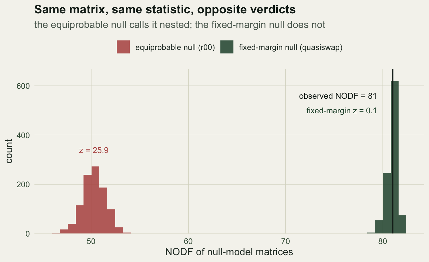
Why the nulls disagree
The equiprobable null generates matrices with roughly equal row and column totals, because it scatters occurrences at random. Real communities are nothing like that: some sites are rich and some poor, some species common and some rare. Compared against a backdrop of even matrices, any community with uneven totals looks nested, whether or not the cells are arranged in a genuinely nested way. The r00 test is therefore mostly detecting that richness and prevalence vary, which is not news.
The fixed-margin null removes that confound. By holding every total fixed, it asks a sharper question: given these exact site richnesses and species prevalences, is the arrangement of cells more nested than chance? For this community the answer is no. The nestedness is a by-product of the uneven totals and adds nothing beyond them, which is why the observed value lands in the middle of the fixed-margin distribution. This is the recurring finding of the null-model literature: much reported nestedness dissolves once the marginal totals are respected (Ulrich and colleagues 2009). A high NODF under a liberal null is common; nestedness beyond the marginals is rare.
The practical rule is short. Report NODF as a description if you like, but test it against a fixed-margin null such as quasiswap or curveball, and treat any nestedness result built on an equiprobable null with suspicion.
Nestedness is not the only community pattern
Two neighbouring ideas are easy to confuse with the NODF pattern. The first is the nestedness-resultant component of beta diversity in the Baselga framework, often written as the nestedness part of a Sorensen split. That is a dissimilarity quantity describing how much of the compositional difference between sites comes from richness differences rather than replacement, and it is computed and interpreted quite separately from a NODF matrix score. A community can register on one and not the other.
The second is co-occurrence, the tendency of species pairs to avoid one another, summarised by the C-score. That is the mirror image of nestedness: instead of subsets it looks for checkerboards, and it runs through the same oecosimu machinery with the same warnings about null-model choice. Both live in vegan, and both reward the same caution about what the null holds fixed.
What to take away
NODF gives you a clean, bounded number for how nested a community is, and vegan computes it in one call. The number alone settles nothing. Its significance depends entirely on the null model, and the honest choice, a fixed-margin null, usually reveals that nestedness is a restatement of uneven richness and prevalence rather than a separate process. Compute NODF, test it against quasiswap, and read the result as a statement about the marginals unless it clears that stricter bar.
References
Almeida-Neto, M., Guimaraes, P., Guimaraes, P.R., Loyola, R.D. and Ulrich, W. 2008. Oikos 117(8):1227-1239 (10.1111/j.0030-1299.2008.16644.x).
Ulrich, W., Almeida-Neto, M. and Gotelli, N.J. 2009. Oikos 118(1):3-17 (10.1111/j.1600-0706.2008.17053.x).