library(vegan)
library(ggplot2)

theme_te <- function(base_size = 12) {
  theme_minimal(base_size = base_size) +
    theme(
      plot.background  = element_rect(fill = "#f5f4ee", colour = NA),
      panel.background = element_rect(fill = "#f5f4ee", colour = NA),
      panel.grid.major = element_line(colour = "#dad9ca", linewidth = 0.3),
      panel.grid.minor = element_blank(),
      axis.text   = element_text(colour = "#46604a"),
      axis.title  = element_text(colour = "#2c3a31"),
      plot.title  = element_text(colour = "#16241d", face = "bold"),
      plot.subtitle = element_text(colour = "#5d6b61"),
      strip.text  = element_text(colour = "#16241d", face = "bold"),
      legend.position = "none"
    )
}
forest <- "#275139"; red <- "#b5534e"; faint <- "#5d6b61"Distance decay of community similarity in R
ecology tutorial
R
vegan
beta diversity
biogeography
spatial ecology
Community similarity falls with geographic distance. Fit the negative-exponential decay in R, read the halving distance, and test it honestly with a Mantel permutation.
Two survey plots that sit close together usually share more species than two plots far apart. Plot that pattern, and a curve appears: compositional similarity slides downward as the distance between plots grows. This is the distance-decay relationship, formalised as a quantitative tool by Nekola and White (1999), and it sits at the heart of biogeography and beta diversity. A Mantel test (covered in a separate tutorial) asks only whether distance and dissimilarity are correlated. Distance decay goes further: it fits the shape of the decline, so you can report a rate and compare it across taxa or regions.
This post fits the decay in R, extracts the halving distance (the distance at which similarity drops by half), decides between the two classic functional forms, and then confronts the awkward statistical fact that makes the naive regression untrustworthy.
A spatially structured community
We place 30 plots in a 50 by 50 km landscape and let each of 40 species have a spatial optimum, so abundance falls off with distance from that optimum. Plots near each other draw on overlapping sets of species, which builds in exactly the turnover we want to measure.
set.seed(72)
n <- 30; S <- 40
coords <- data.frame(x = runif(n, 0, 50), y = runif(n, 0, 50))
cx <- runif(S, 0, 50); cy <- runif(S, 0, 50)   # species spatial optima
w  <- 16                                        # niche width (controls turnover)

lambda <- matrix(0, n, S)
for (j in seq_len(S)) {
  d2 <- (coords$x - cx[j])^2 + (coords$y - cy[j])^2
  lambda[, j] <- 14 * exp(-d2 / (2 * w^2))
}
comm <- matrix(rpois(n * S, lambda), n, S)      # site-by-species counts
dim(comm)
[1] 30 40Similarity is one minus Bray-Curtis dissimilarity; geographic distance is the plain Euclidean distance between coordinates. Both are pairwise, so with 30 plots we get 30 times 29 over 2 = 435 pairs.
sim <- 1 - as.numeric(vegdist(comm, "bray"))
geo <- as.numeric(dist(coords))
c(pairs = length(sim), min_sim = round(min(sim), 3), max_sim = round(max(sim), 3))
pairs min_sim max_sim
435.000 0.139 0.809 Fitting the decay and reading the halving distance
Nekola and White found that the most linear description relates the logarithm of similarity to untransformed distance. That is the negative-exponential model: similarity falls by a constant fraction per kilometre. The slope on the log scale is the decay rate, and the halving distance is log(2) divided by its absolute value.
d <- data.frame(geo = geo, sim = sim, logsim = log(sim), loggeo = log(geo))
m_exp <- lm(logsim ~ geo, data = d)

slope_exp <- coef(m_exp)[["geo"]]
half_dist <- log(2) / abs(slope_exp)
r2_exp    <- summary(m_exp)$r.squared
round(c(slope_per_km = slope_exp, halving_km = half_dist, r2 = r2_exp), 3)
slope_per_km halving_km r2
-0.032 21.639 0.840 The similarity drops by about 3.2% per kilometre, and it takes roughly 22 km for two plots to become half as similar as neighbours. The fit explains 84% of the variation in log-similarity.
xx <- seq(min(geo), max(geo), length.out = 100)
curve_df <- data.frame(geo = xx, sim = exp(predict(m_exp, newdata = data.frame(geo = xx))))

ggplot(d, aes(geo, sim)) +
  geom_point(colour = forest, alpha = 0.5, size = 1.7) +
  geom_line(data = curve_df, colour = red, linewidth = 1) +
  geom_vline(xintercept = half_dist, colour = faint, linetype = "dashed", linewidth = 0.4) +
  annotate("text", x = half_dist + 1, y = 0.72,
           label = paste0("halving distance ~ ", round(half_dist, 0), " km"),
           hjust = 0, colour = faint, size = 3.4) +
  labs(x = "geographic distance (km)", y = "compositional similarity (1 - Bray-Curtis)",
       title = "Community similarity decays with distance",
       subtitle = "negative-exponential fit: log(similarity) linear in distance") +
  theme_te()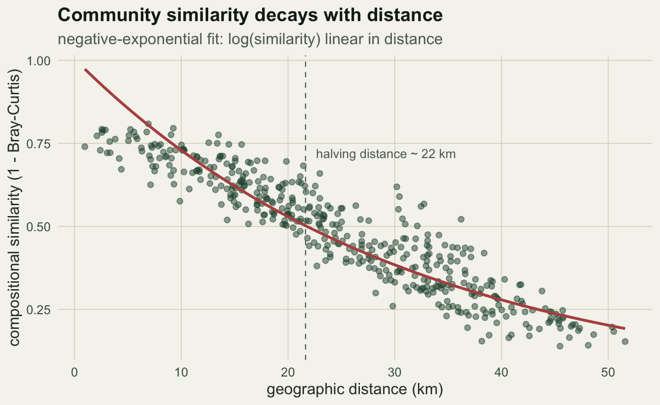
Which functional form?
The other historical option is the power law, where the logarithm of similarity is linear in the logarithm of distance. The two are easy to confuse because both look like straight lines after a log transform, but on different axes. Fit both and compare how straight the cloud actually is.
m_pow  <- lm(logsim ~ loggeo, data = d)
r2_pow <- summary(m_pow)$r.squared
round(c(exp_r2 = r2_exp, power_r2 = r2_pow), 3)
exp_r2 power_r2
0.840 0.636 d1 <- data.frame(x = d$geo, y = d$logsim, form = paste0("negative-exponential (R2 = ", round(r2_exp, 2), ")"))
d2 <- data.frame(x = d$loggeo, y = d$logsim, form = paste0("power law (R2 = ", round(r2_pow, 2), ")"))
ggplot(rbind(d1, d2), aes(x, y)) +
geom_point(colour = forest, alpha = 0.45, size = 1.5) +
geom_smooth(method = "lm", se = FALSE, colour = red, linewidth = 0.9, formula = y ~ x) +
facet_wrap(~form, scales = "free_x") +
labs(x = "predictor (distance, or log distance)", y = "log( similarity )",
title = "Which straight line is the community on?",
subtitle = "the more linear panel is the better-supported decay model") +
theme_te()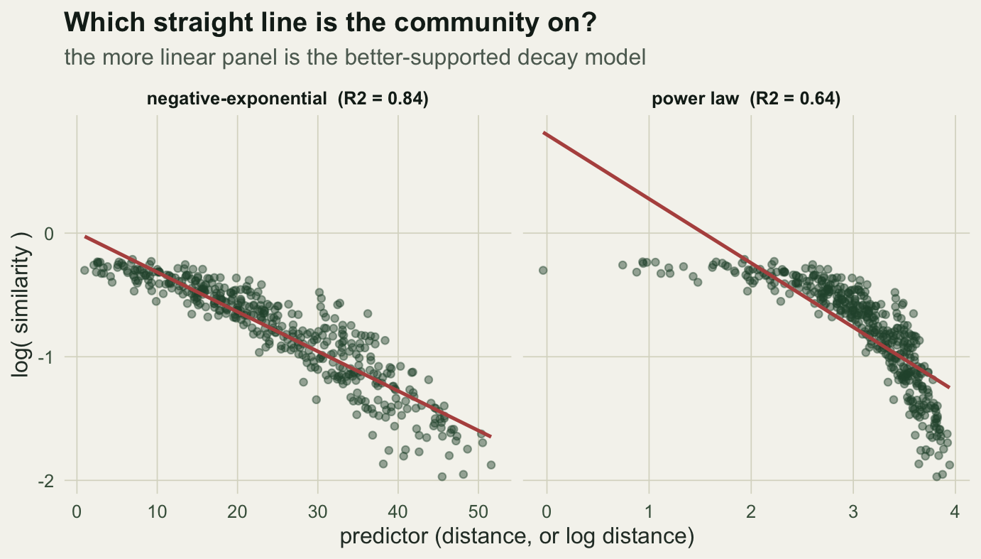
Here the negative-exponential wins, 0.84 against 0.64. That ordering is not a law; it is an empirical question you settle per dataset by comparing fit and residuals. The point is to check rather than assume.
The catch: pairwise distances are not independent
The regression above quietly treated all 435 pairs as independent observations. They are not. Each plot appears in 29 pairs, so one unusual plot nudges dozens of points at once. That inflates the effective sample size and makes ordinary standard errors and p-values far too optimistic. The point estimate of the slope is still a fair summary, but its reported significance is not.
To see how badly this bites, generate communities with no spatial structure at all (composition drawn independently of location) and check how often each method declares a significant decay. With no real signal, an honest test should reject at the nominal 5%.
type1 <- function(nsim, n, S, alpha = 0.05) {
  naive_rej <- 0L; mantel_rej <- 0L
  for (i in seq_len(nsim)) {
    xy <- cbind(runif(n, 0, 50), runif(n, 0, 50))
    cc <- matrix(rpois(n * S, 6), n, S)          # composition independent of space
    ss <- 1 - as.numeric(vegdist(cc, "bray"))
    gg <- as.numeric(dist(xy))
    ok <- ss > 0
    p_ols <- summary(lm(log(ss[ok]) ~ gg[ok]))$coefficients[2, 4]
    naive_rej <- naive_rej + (p_ols < alpha)
    mm <- mantel(dist(xy), vegdist(cc, "bray"), permutations = 499)
    mantel_rej <- mantel_rej + (mm$signif < alpha)
  }
  c(naive = naive_rej / nsim, mantel = mantel_rej / nsim)
}
set.seed(2024)
t1 <- type1(500, 40, 30)
round(100 * t1, 1)
naive mantel
26.8 5.0 The naive regression rejects about 27% of the time when nothing is going on, roughly five times the rate it should. The Mantel permutation, which shuffles whole plots and so respects the dependence, sits right on 5%.
t1df <- data.frame(
  method = factor(c("naive OLS on\nthe 780 pairs", "Mantel\npermutation"),
                  levels = c("naive OLS on\nthe 780 pairs", "Mantel\npermutation")),
  rate = 100 * c(t1[["naive"]], t1[["mantel"]]))

ggplot(t1df, aes(method, rate, fill = method)) +
  geom_col(width = 0.6) +
  geom_hline(yintercept = 5, colour = faint, linetype = "dashed", linewidth = 0.5) +
  annotate("text", x = 2.35, y = 7, label = "nominal 5%", colour = faint, size = 3.3, hjust = 1) +
  geom_text(aes(label = paste0(round(rate, 1), "%")), vjust = -0.4, colour = "#16241d", size = 4) +
  scale_fill_manual(values = c(red, forest)) +
  scale_y_continuous(limits = c(0, 32), expand = expansion(mult = c(0, 0.05))) +
  labs(x = NULL, y = "false-positive rate (no real decay)",
       title = "Pairwise dissimilarities are not independent",
       subtitle = "under no spatial structure, the naive regression rejects far too often") +
  theme_te()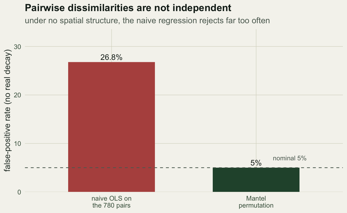
Testing the real decay properly
For the structured community, the honest test is the Mantel correlation between the geographic distance matrix and the Bray-Curtis dissimilarity matrix, with significance from permutations. A positive correlation means dissimilarity rises with distance, which is decay.
set.seed(101)
mt <- mantel(dist(coords), vegdist(comm, "bray"), method = "pearson", permutations = 999)
round(c(mantel_r = mt$statistic, p = mt$signif), 3)
mantel_r p
0.936 0.001 The signal here is real and strong: a Mantel r of 0.94 with a permutation p of 0.001. So use the fitted curve and the halving distance to describe the decay, and lean on the permutation, not the regression p-value, to defend that it is more than noise. The slope is your effect size; the Mantel test is your significance.
What to take away
Distance decay turns a vague sense that “nearby is more similar” into two numbers you can report and compare: a decay rate and a halving distance. Fit the negative-exponential form first, since it is usually the most linear, but compare it against the power law before committing. Above all, remember that a matrix of pairwise similarities carries far less information than its number of entries suggests. Quote the curve from the regression, but let a Mantel permutation carry the hypothesis test.
References
Nekola, J.C. and White, P.S. 1999. Journal of Biogeography 26(4):867-878 (10.1046/j.1365-2699.1999.00305.x).
Soininen, J., McDonald, R. and Hillebrand, H. 2007. Ecography 30(1):3-12 (10.1111/j.0906-7590.2007.04817.x).