library(spdep)
library(ggplot2)

te_paper  <- "#f5f4ee"
te_ink    <- "#16241d"
te_body   <- "#2c3a31"
te_forest <- "#275139"
te_rust   <- "#b5534e"
te_gold   <- "#c9b458"
te_line   <- "#dad9ca"

theme_datasheet <- function() {
  theme_minimal(base_size = 12) +
    theme(plot.background  = element_rect(fill = te_paper, colour = NA),
          panel.background = element_rect(fill = te_paper, colour = NA),
          panel.grid.major = element_line(colour = te_line, linewidth = 0.3),
          panel.grid.minor = element_blank(),
          text             = element_text(colour = te_body),
          plot.title       = element_text(colour = te_ink, face = "bold"),
          plot.subtitle    = element_text(colour = te_body),
          axis.text        = element_text(colour = te_body))
}Moran’s I on residuals: moran.test or lm.morantest
R
spdep
spatial
autocorrelation
regression
model checking
ecology tutorial
Residuals of a model with smooth predictors have a lower null mean than raw data. Why moran.test and moran.mc lose size and power there, and lm.morantest in R.
A hundred and fifty vegetation plots lie scattered over a limestone plateau, and the response is the log of shrub cover. The model has an intercept, one plot-level covariate, and a handful of Moran eigenvector maps added to take up the broad spatial trend. The last line of the script is the check that spatial tutorials teach: Moran’s I on the residuals, with moran.test(residuals(fit), lw) or its permutation twin moran.mc(). A p-value well above 0.05 comes back, and the residuals are declared spatially clean.
That line asks the wrong question. moran.test() treats whatever vector it is given as raw data, and under its null hypothesis the expected value of I is minus one over (n minus one), the value for independent observations of the statistic Moran (1950) introduced. Regression residuals are not raw data: they are the part of the response that is orthogonal to every column of the design matrix, and when those columns are themselves smooth maps the residuals are forced to be rough. Their Moran’s I has a lower mean under the null, and a test centred on the raw-data value then rejects too rarely. Cliff and Ord (1972) worked out the mean and variance of I for least squares residuals, and spdep ships that version as lm.morantest(). None of this is new. What this post adds is a measurement of how much the difference matters once the model carries several spatial predictors.
Three posts on this site run the raw-data null on residuals. Spatial autocorrelation and Moran’s I in R tests the residuals of a one-predictor and a two-predictor model with moran.mc(residuals(m1), lw, nsim = 999), and closes by recommending the permutation test over the normal approximation for irregular points. Moran eigenvector spatial filtering writes its own moran_test() with EI <- -1 / (n - 1) and uses it as the stopping rule for forward selection of up to 25 maps; the rule is applied to the residuals of lm(y ~ x + maps) on Poisson counts, while the reported diagnostic uses Pearson residuals of the Poisson GLM. Checking a spatial regression reuses the same function and the same loop. The first post is where the difference is smallest, with one or two predictors; the second and third are where it is largest. Permutation nulls that keep the map found a site shuffle rejecting too often when it tests the association of two smooth maps; on residuals the shuffle errs the other way.
One plot layout, one graph, a set of maps
The plots are placed uniformly at random in a ten by ten kilometre square. Each plot is joined to its six nearest neighbours, the graph is made symmetric, and the weights are row standardised, which is the style = "W" default of most ecological scripts. The Moran eigenvector maps are the eigenvectors of the doubly centred binary adjacency matrix (Dray, Legendre and Peres-Neto 2006), built as in the eigenvector filtering post and sorted from the broadest pattern down. The plot-level covariate is drawn without any spatial structure.
n_plot <- 150
k_nn   <- 6
set.seed(4102)
plot_xy <- cbind(east = runif(n_plot, 0, 10), north = runif(n_plot, 0, 10))
nb_knn  <- make.sym.nb(knn2nb(knearneigh(plot_xy, k = k_nn)))
lw_knn  <- nb2listw(nb_knn, style = "W")
w_mat   <- listw2mat(lw_knn)
u_mat   <- (w_mat + t(w_mat)) / 2
b_mat   <- nb2mat(nb_knn, style = "B")
cen_mat <- diag(n_plot) - 1 / n_plot
mem_eig <- eigen(cen_mat %*% b_mat %*% cen_mat, symmetric = TRUE)
mem_all <- mem_eig$vectors[, mem_eig$values > 1e-8]
mem_moran <- colSums(mem_all * (w_mat %*% mem_all))
canopy  <- rnorm(n_plot)
stopifnot(abs(sum(w_mat) - n_plot) < 1e-9)

design_mem <- function(n_map) cbind(1, canopy, mem_all[, seq_len(n_map)])
n_link  <- sum(card(nb_knn))
n_pos   <- ncol(mem_all)
The symmetric graph has 1086 directed links, between 6 and 13 neighbours per plot, and 49 maps with positive eigenvalues. The broadest map has a Moran’s I of 0.96 under the row standardised weights, and the sixteenth 0.63.
The residual null has its own mean
With row standardised weights the sum of all weights equals n, and Moran’s I of a centred vector e is simply I = e'We / e'e. For least squares residuals, e = M y with M = I - X (X'X)^-1 X', and under the null of independent normal errors e is M times a spherical normal vector. The ratio e'We / e'e is then independent of its denominator, so its mean is the ratio of the two means, and with tr(M) = n - k that gives
E[I] = tr(M W) / (n - k),
where k is the number of columns of X. This is the Cliff and Ord expectation, and it is what lm.morantest() reports as “Expectation”. Two special cases make it readable. The weights have a zero diagonal, so tr(W) = 0 and tr(M W) = -tr(H W), with H the hat matrix. Writing H through an orthonormal basis of the columns of X, tr(H W) is the sum of q'Wq over the basis vectors: the intercept column contributes exactly one, which with k = 1 gives the familiar minus one over (n minus one). Every other column contributes its own Moran-type autocorrelation. For a design of the intercept and m eigenvector maps, which are orthonormal and orthogonal to the intercept, the expectation is -(1 + I_1 + ... + I_m) / (n - 1 - m), where I_j is the Moran’s I of map j. Adding one more map lowers the expected residual I by about its own Moran’s I divided by (n - k) (exactly, by its Moran’s I minus the current expectation, divided by n - k - 1), which for the broadest maps is close to one over (n - k); a column with no spatial structure moves it by next to nothing.
res_null <- function(X) {
  k_col <- ncol(X)
  m_mat <- diag(n_plot) - X %*% solve(crossprod(X), t(X))
  mu    <- m_mat %*% u_mat
  e_res <- sum(diag(mu)) / (n_plot - k_col)
  v_res <- (2 * sum(mu * t(mu)) + sum(diag(mu))^2) /
    ((n_plot - k_col) * (n_plot - k_col + 2)) - e_res^2
  list(m_mat = m_mat, e_res = e_res, v_res = v_res, k_col = k_col)
}
e_raw <- -1 / (n_plot - 1)
s0 <- sum(w_mat); s1 <- 0.5 * sum((w_mat + t(w_mat))^2)
s2 <- sum((rowSums(w_mat) + colSums(w_mat))^2)
v_raw <- function(b2) {
  nn <- n_plot
  (nn * ((nn^2 - 3 * nn + 3) * s1 - nn * s2 + 3 * s0^2) -
     b2 * ((nn^2 - nn) * s1 - 2 * nn * s2 + 6 * s0^2)) /
    ((nn - 1) * (nn - 2) * (nn - 3) * s0^2) - e_raw^2
}
moran_cols <- function(r_mat) colSums(r_mat * (w_mat %*% r_mat)) / colSums(r_mat^2)

set.seed(611); y_chk <- rnorm(n_plot)
x_chk   <- design_mem(8)
fit_chk <- lm(y_chk ~ x_chk - 1); r_chk <- residuals(fit_chk)
lmt_chk <- lm.morantest(fit_chk, lw_knn); mt_chk <- moran.test(r_chk, lw_knn)
nul_chk <- res_null(x_chk)
b2_chk  <- n_plot * sum(r_chk^4) / sum(r_chk^2)^2
est_l <- lmt_chk$estimate; est_m <- mt_chk$estimate
stopifnot(abs(est_l[["Expectation"]] - nul_chk$e_res) < 1e-12, abs(est_l[["Variance"]] - nul_chk$v_res) < 1e-12,
  abs(est_m[["Expectation"]] - e_raw) < 1e-15, abs(est_m[["Variance"]] - v_raw(b2_chk)) < 1e-12,
  abs(est_l[["Observed Moran I"]] - moran_cols(matrix(r_chk))) < 1e-12,
  isTRUE(formals(moran.test)$randomisation), identical(formals(moran.test)$alternative, "greater"),
  identical(formals(lm.morantest)$alternative, "greater"))

x_only   <- cbind(1, mem_all[, 1:16])
e_decomp <- -(1 + sum(mem_moran[1:16])) / (n_plot - ncol(x_only))
e_plus17 <- e_decomp - (mem_moran[17] - e_decomp) / (n_plot - ncol(x_only) - 1)
stopifnot(abs(res_null(x_only)$e_res - e_decomp) < 1e-12,
          abs(res_null(cbind(x_only, mem_all[, 17]))$e_res - e_plus17) < 1e-12)
spdep_ver <- as.character(packageVersion("spdep"))
The chunk checks the hand version against spdep 1.4.2 to machine precision: on one fitted model with eight maps, lm.morantest() reports an expectation of -0.0598, identical to the trace formula, while moran.test() on the same residuals reports -0.0067, the raw-data value, whatever the vector is. The decomposition matches as well: for the intercept and the first sixteen maps alone, without the covariate, it gives -0.1078 from the sum of the maps’ own Moran’s I, and adding a seventeenth map moves it by exactly the increment above. The stopifnot() line also records the defaults this post relies on, randomisation = TRUE and a one-sided alternative of "greater" in both functions; they are the same in the current development source of spdep (version 1.4-3 on GitHub), where the expectation line of moran.test() is still EI <- (-1) / wc$n1.
map_grid <- c(0, 2, 4, 8, 12, 16)
n_rep    <- 4000
set.seed(8830)
eps_null <- matrix(rnorm(n_plot * n_rep), n_plot)
noise_cols <- matrix(rnorm(n_plot * max(map_grid)), n_plot)
trend_deg  <- 1:4

fam_row <- function(X, family, n_extra) {
  nul   <- res_null(X)
  i_sim <- moran_cols(nul$m_mat %*% eps_null)
  data.frame(family = family, n_extra = n_extra, e_res = nul$e_res,
             sim_mean = mean(i_sim), sim_se = sd(i_sim) / sqrt(n_rep))
}
fam_tab <- rbind(
  do.call(rbind, lapply(map_grid, function(m) fam_row(design_mem(m), "eigenvector maps", m))),
  do.call(rbind, lapply(map_grid, function(m)
    fam_row(cbind(1, canopy, noise_cols[, seq_len(m)]), "unstructured covariates", m))),
  do.call(rbind, lapply(trend_deg, function(d)
    fam_row(cbind(1, canopy, poly(plot_xy[, 1], plot_xy[, 2], degree = d)),
            "trend surface", d * (d + 3) / 2))))
fam_z   <- max(abs(fam_tab$sim_mean - fam_tab$e_res) / fam_tab$sim_se)
e_map16 <- fam_tab$e_res[fam_tab$family == "eigenvector maps" & fam_tab$n_extra == 16]
e_noi16 <- fam_tab$e_res[fam_tab$family == "unstructured covariates" & fam_tab$n_extra == 16]
e_tr14  <- fam_tab$e_res[fam_tab$family == "trend surface" & fam_tab$n_extra == 14]
sd_raw  <- sqrt(v_raw(3)); shift_sd <- (e_raw - e_map16) / sd_raw

n_layout <- 20; set.seed(2213)
layout_e <- vapply(seq_len(n_layout), function(i) {
  xy_i <- cbind(runif(n_plot, 0, 10), runif(n_plot, 0, 10))
  nb_i <- make.sym.nb(knn2nb(knearneigh(xy_i, k = k_nn)))
  w_i  <- listw2mat(nb2listw(nb_i, style = "W"))
  b_i  <- nb2mat(nb_i, style = "B")
  ev_i <- eigen(cen_mat %*% b_i %*% cen_mat, symmetric = TRUE)$vectors[, 1:16]
  x_i  <- cbind(1, rnorm(n_plot), ev_i)
  m_i  <- diag(n_plot) - x_i %*% solve(crossprod(x_i), t(x_i))
  sum(diag(m_i %*% w_i)) / (n_plot - ncol(x_i))
}, numeric(1))
Three families of extra columns were added to the intercept and the covariate: the broadest eigenvector maps, the terms of a polynomial trend surface in the coordinates of degree one to four, and columns of pure noise. Over 4000 null datasets the simulated mean of the residual I agrees with the trace formula in every design, to within 1.1 Monte Carlo standard errors at worst. With sixteen maps the expectation is -0.1076, against -0.0067 for raw data; a quartic trend surface with fourteen terms gives -0.0774; sixteen noise columns give -0.0053. The gap between the sixteen-map value and the raw-data value is 2.4 times the standard deviation that moran.test() itself attaches to I for normal data, so the shift is large against the spread of the null, not a detail of its centre. Across 20 further random layouts of the same size and graph, the sixteen-map expectation ranges from -0.1115 to -0.1066.
fam_plot <- fam_tab
fam_plot$family <- factor(fam_plot$family,
  levels = c("unstructured covariates", "trend surface", "eigenvector maps"))
ggplot(fam_plot, aes(n_extra, e_res, colour = family)) +
  geom_hline(yintercept = e_raw, linetype = "dashed", colour = te_body, linewidth = 0.6) +
  geom_line(linewidth = 0.9) +
  geom_point(aes(y = sim_mean), size = 2.4) +
  annotate("text", x = 16, y = e_raw, vjust = 1.8, hjust = 1, size = 3.4,
           colour = te_body, label = "moran.test: -1/(n - 1)") +
  scale_colour_manual(values = c(te_gold, te_forest, te_rust), name = NULL) +
  scale_x_continuous(breaks = map_grid) +
  labs(x = "extra columns in the model (beyond intercept and covariate)",
       y = "expected residual Moran's I",
       title = "Smooth predictors pull the residual null down",
       subtitle = "150 plots, symmetric 6-nearest-neighbour graph, row standardised") +
  theme_datasheet() +
  theme(legend.position = "bottom")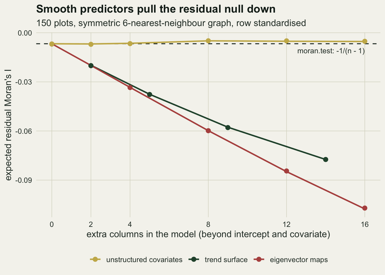
What the raw-data null does to size and power
A null centred too high, and with many maps also too wide, makes a one-sided test reject too rarely. The simulation below fits the model with zero to sixteen maps and applies three tests to the same residuals: the moran.test() default, the moran.mc() permutation test in the next section, and lm.morantest(). Under the null the errors are independent normal; under the alternative they come from a simultaneous autoregressive error process with a coefficient of 0.4 on the same weights. The coefficient and the replication of 4000 datasets per cell were fixed before the first run. The residuals do not depend on the regression coefficients, because M X = 0, so only the errors need to be drawn.
rho_sar <- 0.4
sar_inv <- solve(diag(n_plot) - rho_sar * w_mat)
set.seed(3907)
eps_sar <- sar_inv %*% matrix(rnorm(n_plot * n_rep), n_plot)

rate_cell <- function(n_map, arm) {
  nul   <- res_null(design_mem(n_map))
  r_mat <- nul$m_mat %*% (if (arm == "size") eps_null else eps_sar)
  i_obs <- moran_cols(r_mat)
  b2    <- n_plot * colSums(r_mat^4) / colSums(r_mat^2)^2
  p_raw <- pnorm((i_obs - e_raw) / sqrt(v_raw(b2)), lower.tail = FALSE)
  p_res <- pnorm((i_obs - nul$e_res) / sqrt(nul$v_res), lower.tail = FALSE)
  list(tab = data.frame(n_map = n_map, arm = arm, test = c("moran.test", "lm.morantest"),
                        rate = c(mean(p_raw < 0.05), mean(p_res < 0.05))),
       p_raw = p_raw, p_res = p_res)
}
cells <- expand.grid(n_map = map_grid, arm = c("size", "power"), stringsAsFactors = FALSE)
cell_out <- lapply(seq_len(nrow(cells)), function(i) rate_cell(cells$n_map[i], cells$arm[i]))
rate_tab <- do.call(rbind, lapply(cell_out, `[[`, "tab"))
rate_tab$se <- sqrt(rate_tab$rate * (1 - rate_tab$rate) / n_rep)

chk_cell <- cell_out[[which(cells$n_map == 8 & cells$arm == "power")]]
chk_p <- t(vapply(1:5, function(j) { y_j <- eps_sar[, j]; f_j <- lm(y_j ~ x_chk - 1)
  c(moran.test(residuals(f_j), lw_knn)$p.value, lm.morantest(f_j, lw_knn)$p.value) }, numeric(2)))
stopifnot(max(abs(chk_p[, 1] - chk_cell$p_raw[1:5])) < 1e-10,
          max(abs(chk_p[, 2] - chk_cell$p_res[1:5])) < 1e-10)

get_rate <- function(m, a, tst) rate_tab$rate[rate_tab$n_map == m & rate_tab$arm == a & rate_tab$test == tst]
se_05 <- sqrt(0.05 * 0.95 / n_rep)
lmt_size <- rate_tab$rate[rate_tab$arm == "size" & rate_tab$test == "lm.morantest"]
nul16 <- res_null(design_mem(16)); r_16 <- nul16$m_mat %*% eps_sar; sd_res16 <- sqrt(nul16$v_res)
p_centre <- pnorm((moran_cols(r_16) - nul16$e_res) /
  sqrt(v_raw(n_plot * colSums(r_16^4) / colSums(r_16^2)^2)), lower.tail = FALSE)
pow_centre <- mean(p_centre < 0.05)
The chunk checks the vectorised p-values against five calls each of moran.test() and lm.morantest() on fitted lm objects; they agree to ten decimal places. With no maps in the model the two tests are the same test for practical purposes: 0.057 and 0.057 under the null, 0.894 and 0.894 under the autoregressive errors. With eight maps the moran.test() default rejects a true null in 0.0013 of datasets and detects the autoregressive errors in 0.242; lm.morantest() on the same residuals gives 0.062 and 0.717. With sixteen maps the default rejects 0 of the 4000 null datasets and 4 of the autocorrelated ones, while lm.morantest() gives 0.057 and 0.485. The Monte Carlo standard error of a rate near five per cent is 0.0034, and no larger than 0.0079 for any rate. Two things fall with the number of maps and they should be kept apart. The power of lm.morantest() falls too, from 0.894 to 0.485, because the maps absorb part of the autocorrelation the errors carry: there is less of it left in the residuals to find. That loss is real and no residual test can recover it. The rest of the gap at sixteen maps, from 0.485 down to 0.0010, is the raw-data null, and both of its moments are wrong. Moving only its centre to the residual expectation brings the power back to 0.249; correcting its spread as well, a standard deviation of 0.0422 for normal data against 0.0281 for the residual null, takes it the rest of the way. At that point a residual check with the default test can hardly fail: it passes independent errors and autocorrelated ones alike.
The size of lm.morantest() is a little above five per cent in all six designs, between 0.056 and 0.062. The six rates share the same simulated errors, so they are one measurement, not six, and it sits 1.7 to 3.6 Monte Carlo standard errors above the nominal level. spdep also carries an exact version, lm.morantest.exact(), which computes the null distribution of the ratio of quadratic forms as Tiefelsdorf and Boots (1995) set it out. The chunk below compares both versions with p-values read directly off the 4000 simulated null statistics of the same design.
n_exact <- 200
exact_cmp <- do.call(rbind, lapply(c(0, 16), function(n_map) {
  x_d   <- design_mem(n_map)
  nul   <- res_null(x_d)
  i_ref <- moran_cols(nul$m_mat %*% eps_null)
  skew  <- mean((i_ref - mean(i_ref))^3) / sd(i_ref)^3
  data.frame(n_map = n_map, skew = skew, t(vapply(seq_len(n_exact), function(j) {
    y_j <- eps_null[, j]
    c(p_exact  = lm.morantest.exact(lm(y_j ~ x_d - 1), lw_knn)$p.value,
      p_normal = pnorm((i_ref[j] - nul$e_res) / sqrt(nul$v_res), lower.tail = FALSE),
      p_sim    = mean(i_ref[-j] >= i_ref[j]))
  }, numeric(3))))
}))
tail_cmp  <- exact_cmp[exact_cmp$p_sim < 0.2, ]
se_tail   <- sqrt(tail_cmp$p_sim * (1 - tail_cmp$p_sim) / (n_rep - 1))
z_exact   <- max(abs(tail_cmp$p_exact - tail_cmp$p_sim) / se_tail)
z_norm    <- max((tail_cmp$p_sim - tail_cmp$p_normal) / se_tail)
stopifnot(z_norm == max(abs(tail_cmp$p_normal - tail_cmp$p_sim) / se_tail))
se_p02    <- sqrt(0.02 * 0.98 / (n_rep - 1))
small_ex  <- exact_cmp$p_exact < 0.05
n_small   <- tapply(small_ex, exact_cmp$n_map, sum)
ratio_ne  <- tapply((exact_cmp$p_normal / exact_cmp$p_exact)[small_ex], exact_cmp$n_map[small_ex], mean)
skew_ref  <- tapply(exact_cmp$skew, exact_cmp$n_map, mean)
Over the first 200 null datasets with no maps and with sixteen, 83 have a simulated p-value below 0.2, the region where a decision is made. Each simulated p-value has its own Monte Carlo standard error, about 0.0022 near p = 0.02. In those units the exact p-values differ from the simulated ones by at most 2.0 standard errors, while the largest gap of the normal approximation is 4.0 standard errors, with its p-value below the simulated one. The simulated p-values of a design all come from one reference sample, so this is one deviation of one empirical distribution, not many independent ones. The two computed versions can also be set against each other, which involves no simulation at all: where the exact p-value is below 0.05 (10 datasets with no maps, 11 with sixteen), the normal p-value is on average 0.57 and 0.59 times the exact one. The null distribution of I is skewed to the right, with a skewness of 0.31 and 0.30 over the simulated statistics, and a normal curve with the same mean and variance puts too little weight in the upper tail. That is where the small excess in the size of lm.morantest() comes from, and it is there with no maps at all: it belongs to the normal approximation, not to the residual null.
The permutation route has the same null
moran.mc() looks like the safer choice, and the Moran’s I post recommends it for irregular points. It is not a different null. It shuffles the residuals across plots and recomputes I each time, which asks what I would look like if the same values had landed on the plots in random order. For any centred vector the average of I over all orderings is exactly minus one over (n minus one): every pair of distinct positions is equally likely to receive every pair of distinct values, and the sum of all cross products of centred values is minus their sum of squares. The shuffle forgets that the residuals were built to be orthogonal to the maps, which is exactly the constraint that moved their null.
perm_mc <- function(r, nsim) {
  pm    <- vapply(seq_len(nsim), function(i) sample(r), numeric(n_plot))
  i_all <- c(colSums(pm * (w_mat %*% pm)) / sum(r^2), sum(r * (w_mat %*% r)) / sum(r^2))
  rk    <- rank(i_all)[nsim + 1]
  list(p = (max(nsim - rk, 0) + 1) / (nsim + 1), i_perm = i_all[seq_len(nsim)])
}
r_one  <- as.numeric(nul16$m_mat %*% eps_null[, 1])
set.seed(71); mc_one <- moran.mc(r_one, lw_knn, nsim = 999)
set.seed(71); hand_one <- perm_mc(r_one, 999)
stopifnot(abs(mc_one$p.value - hand_one$p) < 1e-12,
          max(abs(mc_one$res[1:999] - hand_one$i_perm)) < 1e-12)
perm_mean <- mean(hand_one$i_perm)
i_one     <- sum(r_one * (w_mat %*% r_one)) / sum(r_one^2)
p_one_lmt <- pnorm((i_one - nul16$e_res) / sqrt(nul16$v_res), lower.tail = FALSE)
null16_i  <- moran_cols(nul16$m_mat %*% eps_null)

n_perm_rep <- 500; n_perm_sim <- 199; perm_maps <- c(0, 8, 16); set.seed(5150)
perm_tab <- do.call(rbind, lapply(perm_maps, function(n_map) {
  m_mat <- res_null(design_mem(n_map))$m_mat
  p_n <- vapply(seq_len(n_perm_rep), function(j)
    perm_mc(as.numeric(m_mat %*% eps_null[, j]), n_perm_sim)$p, numeric(1))
  p_a <- vapply(seq_len(n_perm_rep), function(j)
    perm_mc(as.numeric(m_mat %*% eps_sar[, j]), n_perm_sim)$p, numeric(1))
  data.frame(n_map = n_map, arm = c("size", "power"), test = "moran.mc on residuals",
             rate = c(mean(p_n < 0.05), mean(p_a < 0.05)))
}))
perm_tab$se <- sqrt(perm_tab$rate * (1 - perm_tab$rate) / n_perm_rep)
get_perm <- function(m, a) perm_tab$rate[perm_tab$n_map == m & perm_tab$arm == a]
The hand-written shuffle reproduces moran.mc() exactly when both start from the same random seed: the same 999 permuted statistics and the same p-value. Take one null dataset fitted with sixteen maps. Its residual I is -0.1104. The shuffled values average -0.0063, next to the exact -0.0067, and give a permutation p-value of 0.998; lm.morantest() gives 0.540 for the same residuals, referred to a null centred at -0.1076.
Over 500 datasets per cell, with 199 shuffles each, the permutation test on residuals rejects a true null in 0.052, 0.004 and 0.000 of datasets with zero, eight and sixteen maps, and detects the autoregressive errors in 0.872, 0.216 and 0.000. It tracks the moran.test() default, not lm.morantest().
dens_df <- rbind(
  data.frame(i_val = null16_i, what = "residual I over 4000 null datasets"),
  data.frame(i_val = hand_one$i_perm, what = "999 shuffles of one residual vector"))
ggplot(dens_df, aes(i_val, fill = what, colour = what)) +
  geom_density(alpha = 0.35, linewidth = 0.7) +
  geom_vline(xintercept = c(nul16$e_res, e_raw), linetype = "dashed",
             colour = c(te_forest, te_rust), linewidth = 0.6) +
  geom_vline(xintercept = i_one, colour = te_ink, linewidth = 0.7) +
  scale_fill_manual(values = c(te_rust, te_forest), name = NULL) +
  scale_colour_manual(values = c(te_rust, te_forest), name = NULL) +
  labs(x = "Moran's I", y = "density",
       title = "Shuffling residuals rebuilds the raw-data null",
       subtitle = "dashed green: tr(MW)/(n - k); dashed red: -1/(n - 1)") +
  theme_datasheet() +
  theme(legend.position = "bottom")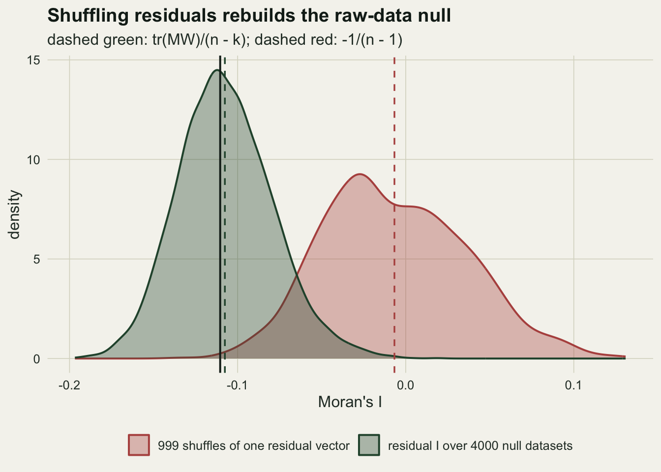
rates_all <- rbind(rate_tab, perm_tab)
rates_all$panel <- factor(ifelse(rates_all$arm == "size", "no autocorrelation (size)",
                                 "autoregressive errors, 0.4 (power)"),
                          levels = c("no autocorrelation (size)", "autoregressive errors, 0.4 (power)"))
rates_all$test <- factor(rates_all$test,
                         levels = c("lm.morantest", "moran.test", "moran.mc on residuals"))
ref_df <- data.frame(panel = factor("no autocorrelation (size)", levels = levels(rates_all$panel)),
                     yint = 0.05)
ggplot(rates_all, aes(n_map, rate, colour = test)) +
  geom_hline(data = ref_df, aes(yintercept = yint), linetype = "dashed",
             colour = te_body, linewidth = 0.5) +
  geom_line(data = rates_all[rates_all$test != "moran.mc on residuals", ], linewidth = 0.9) +
  geom_errorbar(aes(ymin = pmax(rate - 2 * se, 0), ymax = rate + 2 * se),
                width = 0.5, linewidth = 0.5) +
  geom_point(aes(shape = test), size = 2.4) +
  facet_wrap(~ panel, scales = "free_y") +
  scale_colour_manual(values = c(te_forest, te_rust, te_gold), name = NULL) +
  scale_shape_manual(values = c(16, 16, 17), name = NULL) +
  scale_x_continuous(breaks = map_grid) +
  labs(x = "eigenvector maps in the model", y = "rejection rate at 0.05",
       title = "The raw-data null stops detecting anything",
       subtitle = "dashed: the nominal five per cent") +
  theme_datasheet() +
  theme(legend.position = "bottom")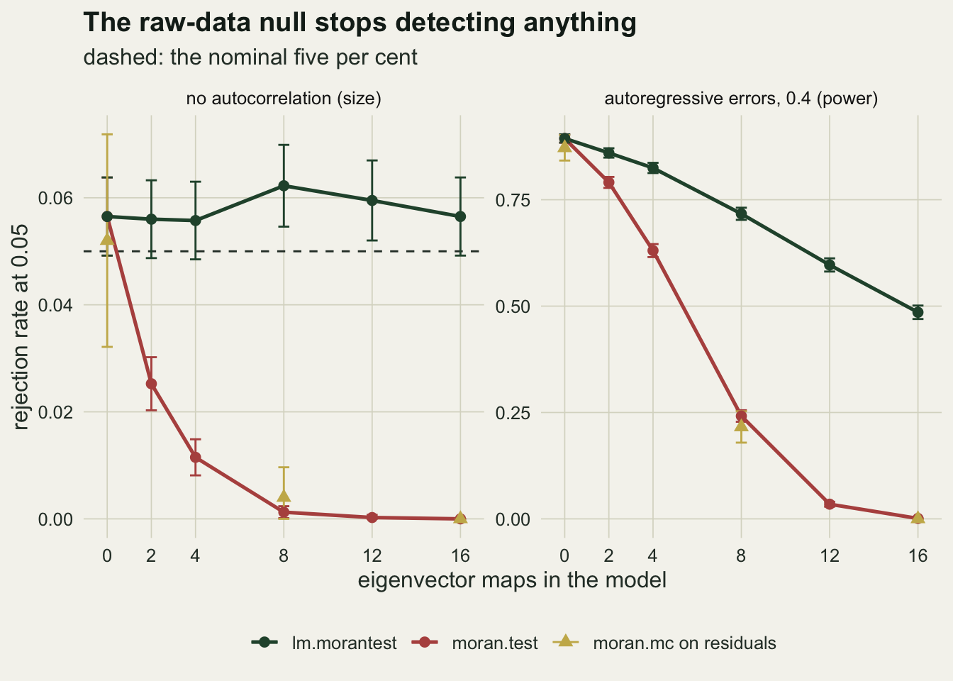
A stopping rule built on the wrong null
The eigenvector filtering post uses the residual test as a stopping rule: add the map most correlated with the residuals, test again, stop when the residual I is no longer significant. A test that rejects too rarely stops the loop early. The simulation below repeats that loop on the plateau layout with a covariate that has no effect on the response but shares the broadest map with an unmeasured smooth field that does, which is the confounded case the filtering post was built for. The candidates are the first 40 maps, the loop is capped at 30, and each of 400 datasets is run twice, once with each test as the rule.
n_sel_rep <- 400
cand_map  <- 1:40
max_map   <- 30
p_raw_one <- function(r) pnorm((moran_cols(matrix(r)) - e_raw) /
  sqrt(v_raw(n_plot * sum(r^4) / sum(r^2)^2)), lower.tail = FALSE)
p_res_one <- function(r, X) { nul <- res_null(X)
  pnorm((moran_cols(matrix(r)) - nul$e_res) / sqrt(nul$v_res), lower.tail = FALSE) }
run_select <- function(y, x, rule) {
  sel <- integer(0)
  repeat {
    X <- cbind(1, x, mem_all[, sel, drop = FALSE])
    r <- as.numeric(y - X %*% qr.coef(qr(X), y))
    p <- if (rule == "raw") p_raw_one(r) else p_res_one(r, X)
    if (p > 0.05 || length(sel) >= max_map) break
    left <- setdiff(cand_map, sel)
    sel  <- c(sel, left[which.max(abs(cor(mem_all[, left], r)))])
  }
  X   <- cbind(1, x, mem_all[, sel, drop = FALSE])
  fit <- lm(y ~ X - 1)
  c(n_map = length(sel), x_fp = summary(fit)$coefficients[2, 4] < 0.05,
    ac_left = p_res_one(residuals(fit), X) < 0.05, capped = length(sel) >= max_map)
}
set.seed(4478)
sel_out <- replicate(n_sel_rep, {
  field <- as.numeric(scale(mem_all[, 1] * rnorm(1, 1, 0.1) +
                              mem_all[, 2:12] %*% rnorm(11, 0, 0.5) + rnorm(n_plot, 0, 0.2)))
  x_conf <- as.numeric(scale(0.6 * mem_all[, 1] / sd(mem_all[, 1]) + rnorm(n_plot)))
  y_sel  <- field + rnorm(n_plot)
  c(run_select(y_sel, x_conf, "raw"), run_select(y_sel, x_conf, "res"),
    ols_fp = summary(lm(y_sel ~ x_conf))$coefficients[2, 4] < 0.05)
})
sel_mean <- rowMeans(sel_out)
sel_raw_k <- sel_out[1, ]
sel_res_k <- sel_out[5, ]
fp_raw <- sel_mean[2]; fp_res <- sel_mean[6]; fp_ols <- sel_mean[9]
left_raw <- sel_mean[3]; left_res <- sel_mean[7]
fp_diff_se <- sd(sel_out[2, ] - sel_out[6, ]) / sqrt(n_sel_rep)
k_diff_se  <- sd(sel_res_k - sel_raw_k) / sqrt(n_sel_rep)
n_capped   <- sum(sel_out[4, ]) + sum(sel_out[8, ])
With the raw-data rule the loop keeps 1.95 maps on average and with the residual rule 2.36, a paired difference with a standard error of 0.03. The cap of 30 maps was reached in 0 of the 800 runs. After the raw-data rule has stopped, lm.morantest() still finds autocorrelation in the final model’s residuals in 0.338 of datasets; after the residual rule the share is 0.000, which is zero by construction, since that rule stops only when the same test passes.
The covariate’s false-positive rate is a different quantity and it barely moves. It is 0.2350 after the raw-data rule and 0.2325 after the residual rule, a paired difference of +0.0025 with a standard error of 0.007, and 0.282 for plain least squares with no maps at all. Both filtered rates are far above five per cent. The correct residual test makes the stopping rule honest about the residuals; it does not repair the inference for a covariate that shares its spatial pattern with an unmeasured driver. That confounding is the limit the eigenvector filtering post states itself, and no choice of residual test reaches it.
k_levels <- 0:max(c(sel_raw_k, sel_res_k))
k_df <- rbind(
  data.frame(n_map = k_levels, share = tabulate(sel_raw_k + 1, length(k_levels)) / n_sel_rep,
             rule = "stop on moran.test (raw-data null)"),
  data.frame(n_map = k_levels, share = tabulate(sel_res_k + 1, length(k_levels)) / n_sel_rep,
             rule = "stop on lm.morantest (residual null)"))
ggplot(k_df, aes(factor(n_map), share, fill = rule)) +
  geom_col(position = position_dodge(width = 0.8), width = 0.75) +
  scale_fill_manual(values = c(te_forest, te_rust), name = NULL) +
  labs(x = "eigenvector maps kept", y = "share of datasets",
       title = "The raw-data rule tends to stop earlier",
       subtitle = "same datasets, same candidate maps, same selection order") +
  theme_datasheet() +
  theme(legend.position = "bottom", legend.direction = "vertical")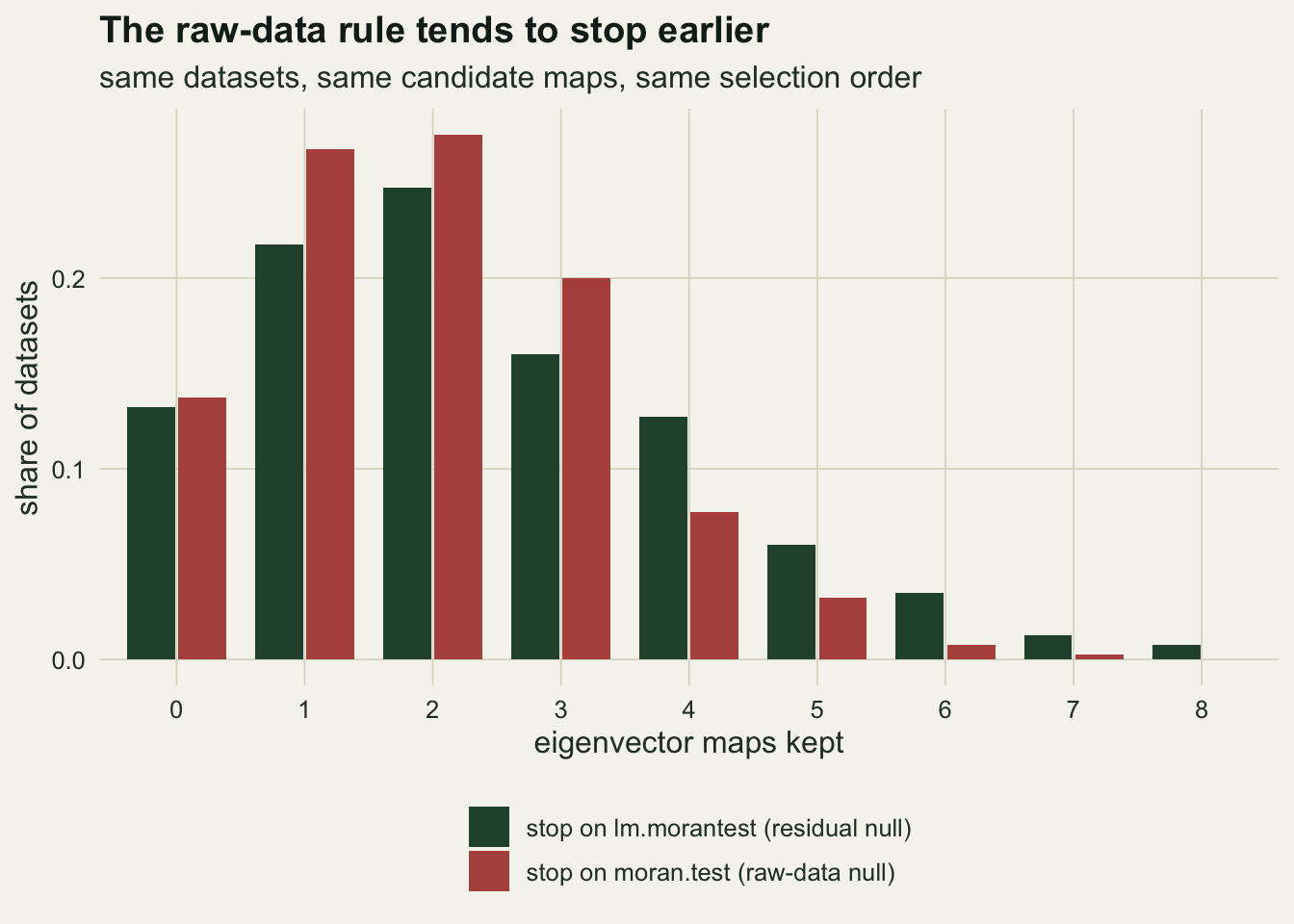
What to report
For residuals of a linear model fitted by least squares, test with lm.morantest(fit, lw) rather than moran.test(residuals(fit), lw) or moran.mc(residuals(fit), lw, nsim). It takes the fitted lm object, not the residual vector, because it needs the design matrix, and it prints the expectation it used. Report that expectation next to the observed I, together with the number of columns in the model and the weights: an observed residual I of zero is a positive deviation when the null mean is -0.108. Where the sample is small or the p-value sits near the threshold, lm.morantest.exact() gives the exact version at little cost; on the design here its tail p-values matched the simulation, while those of the normal approximation ran too small.
With one or two predictors and no smooth terms the three tests agree closely, and a residual check run with moran.test() or moran.mc() reads the same way. The difference grows with every smooth column in the model: eigenvector maps, trend surface terms, spline bases of the coordinates, or environmental layers that are themselves smooth. A model built to remove spatial structure is the worst place for the raw-data null, because that is where the design is smoothest. When the test is a stopping rule, as in eigenvector selection, say which null was used. A rule on the raw-data null stops earlier and can leave detectable residual autocorrelation behind. Neither rule controls the error rate of a confounded covariate, which has to be argued separately.
Honest limits
Everything here is one layout of 150 random plots with one graph, the symmetric six-nearest-neighbour graph with row standardised weights. The expectation was checked over 20 further layouts and moved little, but the rates were measured on one. A binary or distance-weighted graph changes the constants, not the mechanism; the formula applies to any weights.
The Cliff and Ord moments are exact for a linear model with independent normal errors. The eigenvector filtering post applies its stopping rule to lm() residuals of Poisson counts and reports Pearson residuals of a Poisson GLM; for those, the trace formula is an approximation, and the residual null of a GLM depends on its working weights. Nothing here measures how good that approximation is for counts. A parametric bootstrap from the fitted GLM, refitting and recomputing I each time, is the general route there and is not shown.
The size and power study fits the first m maps in a fixed order. Forward selection instead chooses the maps that best match the residuals, and after that choice the residuals are no longer a fixed projection of the errors: even lm.morantest() is not exact after selection, since it treats the selected maps as if they had been fixed in advance. The selection section measures how the two rules behave; it does not claim either one has an exact level.
The autoregressive alternative used one coefficient, 0.4, on the same graph that defines the test. Autocorrelation at a scale the graph does not see, or at a coefficient near zero, gives lower power to every test, and the ranking of the tests was not checked there. The selection study has one confounding structure, one field generator and 40 candidate maps; its false-positive rates belong to that design, and only their failure to differ between the two rules is the point.
References
Moran PAP 1950 Biometrika 37(1-2):17-23 (10.1093/biomet/37.1-2.17)
Cliff AD, Ord JK 1972 Geographical Analysis 4(3):267-284 (10.1111/j.1538-4632.1972.tb00475.x)
Tiefelsdorf M, Boots B 1995 Environment and Planning A 27(6):985-999 (10.1068/a270985)
Dray S, Legendre P, Peres-Neto PR 2006 Ecological Modelling 196(3-4):483-493 (10.1016/j.ecolmodel.2006.02.015)