---
title: "t-tests and ANOVA as linear models in R"
description: "A t-test and a one-way ANOVA are the same linear model. Fit both in R on grassland data, read treatment-coded coefficients, and see why F equals t squared."
date: "2026-06-26 10:00"
categories: [R, linear models, ANOVA, regression, ecology tutorial]
image: thumbnail.png
image-alt: "Vegetation height for three grassland management types, points jittered with group means marked and a dashed line at the grazed mean."
---
Most ecologists meet the t-test and analysis of variance as separate items on a menu: two groups call for one test, three or more groups call for another, and regression is something else again. That menu hides a simpler picture. The t-test, one-way ANOVA, and ordinary regression are the same procedure underneath: a linear model that splits a response into a baseline plus the effect of one or more predictors. Seeing the connection makes the output easier to read, and it is the step that lets you add covariates, interactions, non-normal responses, and random effects later without learning a new test for each situation.
We will use a small grassland dataset: vegetation height measured on plots under three management regimes (grazed, mown, and abandoned). The aim is to compare heights across management, first with two groups and then with three, and to watch the same linear model appear under each classical test.
```{r}
#| include: false
library(ggplot2)
library(dplyr)
paper <- "#f5f4ee"; ink <- "#16241d"; body <- "#2c3a31"
forest <- "#275139"; label <- "#46604a"; faint <- "#5d6b61"; line <- "#dad9ca"
mgmt_cols <- c(Grazed = "#cda23f", Mown = "#2f8f63", Abandoned = "#b5534e")
base_theme <- theme_minimal(base_size = 13) +
theme(plot.background = element_rect(fill = paper, colour = NA),
panel.background = element_rect(fill = paper, colour = NA),
panel.grid.minor = element_blank(),
panel.grid.major = element_line(colour = line, linewidth = 0.3),
axis.title = element_text(colour = body),
axis.text = element_text(colour = faint),
legend.position = "none")
```
## The data
Three management types, twenty plots each, height in centimetres. The figure styling is house style and lives in a hidden setup block; if you want to reproduce the plots, see the [figure export post](../publication-quality-ggplot-figures/) for the theme pattern.
```{r}
set.seed(38)
n  <- 20
mt <- c("Grazed", "Mown", "Abandoned")
veg <- data.frame(
  management = factor(rep(mt, each = n), levels = mt),
  height = c(rnorm(n, 14, 4), rnorm(n, 9, 4), rnorm(n, 24, 5))
)

veg %>%
  group_by(management) %>%
  summarise(n = n(), mean = mean(height), sd = sd(height))
```
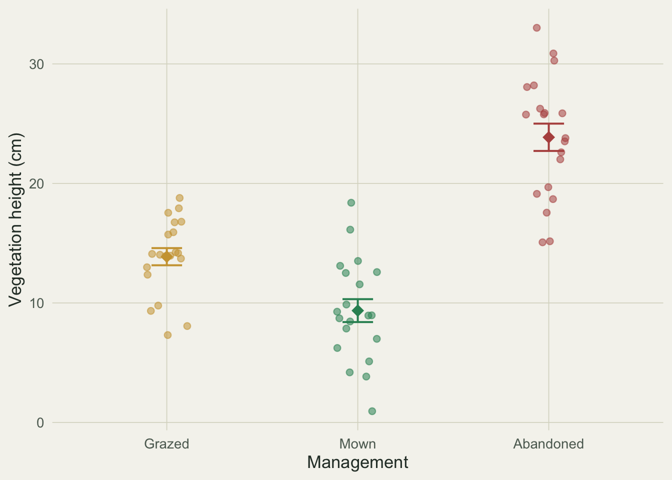
The grazed plots sit near 13.9 cm, mown plots near 9.4 cm, and abandoned plots near 23.9 cm. Those three numbers are the whole story; every model below is a way of comparing them while carrying the right standard errors.
```{r}
#| fig-cap: "Vegetation height by management. Points are plots, diamonds are group means, bars are one standard error."
#| fig-alt: "Jittered points of vegetation height for grazed, mown and abandoned plots, with a diamond and error bar marking each group mean. Abandoned is highest near 24 cm, grazed near 14 cm, mown lowest near 9 cm."
ggplot(veg, aes(management, height, colour = management)) +
  geom_jitter(width = 0.12, height = 0, size = 2, alpha = 0.55) +
  stat_summary(fun.data = mean_se, geom = "errorbar", width = 0.16, linewidth = 0.7) +
  stat_summary(fun = mean, geom = "point", size = 4, shape = 18) +
  scale_colour_manual(values = mgmt_cols) +
  labs(x = "Management", y = "Vegetation height (cm)") +
  base_theme
```
## Two groups: a t-test is a linear model
Take grazed and mown plots and ask whether their mean heights differ. The textbook tool is a two-sample t-test. We use the equal-variance form, because that is the version a linear model fits by default (a single pooled error variance).
```{r}
two <- droplevels(subset(veg, management %in% c("Grazed", "Mown")))
t.test(height ~ management, data = two, var.equal = TRUE)
```
The test reports `t = 3.77` on 38 degrees of freedom and `p = 0.00056`, with group means of 13.9 and 9.4 cm. Now fit a linear model to the same two groups:
```{r}
m2 <- lm(height ~ management, data = two)
summary(m2)$coefficients
```
The two outputs carry the same information in different dress. The intercept, 13.87, is the grazed mean. The `managementMown` coefficient, -4.51, is the difference in means: mown plots are 4.51 cm shorter. The coefficient's t value, -3.77, matches the t-test exactly (the sign only reflects which group is the reference), and so does the p-value. A t-test is a linear model with one predictor that happens to be a two-level factor.
The link runs one step further. For two groups, the ANOVA F statistic is the square of that t value:
```{r}
c(F_from_anova = anova(m2)[1, "F value"],
  t_squared    = summary(m2)$coefficients[2, "t value"]^2)
```
Both are 14.19. The F test and the t test are not two ways of deciding the same question; they are the same arithmetic.
## Three groups: one-way ANOVA is the same model
Add the abandoned plots back. With three groups a t-test no longer applies, and the usual move is a one-way ANOVA. In R that is still `lm`:
```{r}
m <- lm(height ~ management, data = veg)
summary(m)$coefficients
```
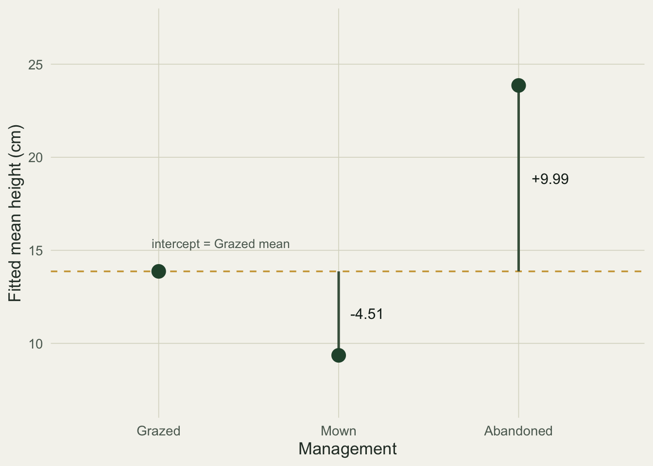
R turns the three-level factor into two columns by treatment coding (also called dummy coding). The first level, grazed, becomes the reference and is folded into the intercept. The other two coefficients are differences from that reference: mown is 4.51 cm shorter, abandoned is 9.99 cm taller. You can read the group means straight off the coefficients by adding each offset to the intercept.
```{r}
model.matrix(m)[c(1, 21, 41), ]
```
Each row of the design matrix is one group. A grazed plot is all zeros after the intercept, so its fitted value is the intercept alone. A mown plot switches on the `managementMown` column, an abandoned plot switches on `managementAbandoned`. The coefficients are the heights of those switches.
```{r}
#| fig-cap: "Treatment coding. The dashed line is the intercept (grazed mean); each coefficient is the signed distance from it to a group mean."
#| fig-alt: "Three fitted group means against a dashed baseline at the grazed mean of about 14 cm. An arrow drops 4.51 cm down to mown and an arrow rises 9.99 cm up to abandoned, labelling the two treatment-coded coefficients."
means_df <- data.frame(management = factor(mt, levels = mt),
                       mean = as.numeric(c(coef(m)[1],
                                           coef(m)[1] + coef(m)[2],
                                           coef(m)[1] + coef(m)[3])))
seg <- subset(means_df, management != "Grazed")
seg$lab <- sprintf("%+.2f", as.numeric(coef(m)[2:3]))

ggplot(means_df, aes(management, mean)) +
  geom_hline(yintercept = coef(m)[1], linetype = "dashed",
             colour = "#cda23f", linewidth = 0.6) +
  geom_segment(data = seg, aes(xend = management, y = coef(m)[1], yend = mean),
               arrow = arrow(length = unit(0.18, "cm")),
               linewidth = 0.9, colour = label) +
  geom_point(size = 4.5, colour = forest) +
  geom_text(data = seg, aes(y = (coef(m)[1] + mean) / 2, label = lab),
            hjust = -0.35, colour = ink, size = 4) +
  scale_x_discrete(limits = mt, expand = expansion(add = c(0.6, 0.7))) +
  annotate("text", x = 1, y = coef(m)[1] + 1.5,
           label = "intercept = Grazed mean", colour = faint, size = 3.4, hjust = 0.05) +
  labs(x = "Management", y = "Fitted mean height (cm)") +
  coord_cartesian(ylim = c(7, 27)) +
  base_theme
```
The omnibus F test asks a single question: is there any difference among the three group means? `anova` on the linear model and `aov` give the identical answer, because `aov` is a wrapper around `lm`:
```{r}
anova(m)
c(aov_F = summary(aov(height ~ management, data = veg))[[1]][1, "F value"],
  lm_F  = anova(m)[1, "F value"])
```
The F statistic is 60.3 on 2 and 57 degrees of freedom, with a p-value near `8.6e-15`. Management accounts for most of the spread in height: the model's R-squared is 0.68. None of this required a separate ANOVA routine.
## One detail worth noticing
The `managementMown` coefficient is -4.51 in both the two-group and three-group models, but its standard error grew from 1.20 to 1.35. The estimate of the difference did not change; the estimate of the error variance did. A linear model pools one residual variance across every group in the model, and the abandoned plots are more variable than the other two. Folding them in raises the pooled variance, which widens the standard error on the grazed-versus-mown contrast even though that contrast never touched the abandoned data. Which groups you include changes the uncertainty, not the point estimate.
This is also why the omnibus test stops where it does. A significant F says the group means are not all equal; it does not say which pairs differ. Answering that calls for planned contrasts or post-hoc comparisons, with attention to the error rate when you make several of them. That is the subject of the [next post on contrasts and post-hoc comparisons](../contrasts-and-post-hoc/).
## Why the equivalence is useful
Once the t-test and ANOVA are linear models, the rest of the toolbox is the same object with more terms. Add a continuous covariate and you have analysis of covariance. Add a second factor and an interaction and you have a factorial design. Swap the normal errors for a Poisson or binomial family and you have a [generalised linear model for counts](../glm-count-data-abundance/) or [presence-absence](../logistic-regression-presence-absence/). Add a random intercept for repeated measures on the same site and you have a [mixed model](../glmm-nested-counts-pseudoreplication/). You never leave the `response ~ predictors` formula; you only change what sits on each side and how the errors are distributed. Learning to read treatment-coded coefficients once pays off across all of them.
## References
Student 1908 Biometrika 6(1):1-25 (10.1093/biomet/6.1.1).
Fisher 1925 Statistical Methods for Research Workers, Oliver and Boyd (no DOI).
Crawley 2013 The R Book, 2nd ed., Wiley (ISBN 978-0-470-97392-9).
Faraway 2014 Linear Models with R, 2nd ed., Chapman and Hall/CRC (ISBN 978-1-4398-8733-2).