library(ggplot2)
library(patchwork)

te_paper  <- "#f5f4ee"
te_ink    <- "#16241d"
te_body   <- "#2c3a31"
te_forest <- "#275139"
te_rust   <- "#b5534e"
te_gold   <- "#c9b458"
te_line   <- "#dad9ca"

theme_datasheet <- function() {
  theme_minimal(base_size = 12) +
    theme(plot.background  = element_rect(fill = te_paper, colour = NA),
          panel.background = element_rect(fill = te_paper, colour = NA),
          panel.grid.major = element_line(colour = te_line, linewidth = 0.3),
          panel.grid.minor = element_blank(),
          text             = element_text(colour = te_body),
          plot.title       = element_text(colour = te_ink, face = "bold"),
          plot.subtitle    = element_text(colour = te_body),
          axis.text        = element_text(colour = te_body))
}Line transects along tracks and avoidance
R
distance sampling
abundance
survey design
model checking
ecology tutorial
Line transects on tracks animals avoid: a half-normal fit can lose over half the density, and the fit test mostly misses the costliest gradients. In R.
A forestry block of spruce and birch holds roe deer and brown hares, and the district wants a density for both. Random lines through the plantation are slow to walk and hard to keep straight, so the observers use the forestry tracks: they are already mapped, the sight lines along them are clear, and a kilometre of track is walked far faster than a kilometre of brash. The distances to every animal seen are measured with a rangefinder, perpendicular to the track, exactly as a line transect survey requires. The analysis fits a half-normal detection function, the histogram looks sensible, and the goodness-of-fit test passes.
The tracks carry timber lorries, dog walkers and the observers themselves, and animals that use the block do not spread evenly up to the verge. That breaks the assumption every distance sampling estimator starts from: that animals are distributed uniformly with respect to the line. This site has said so three times without measuring it. Distance sampling for density in R lists among its assumptions that lines must be placed at random with respect to the animals, not along features that concentrate them. The table in checking a distance sampling model records uniformity with respect to the line as an assumption the distances cannot check, settled only by random placement of the design. Point transect distance sampling closes by saying that no care with the key function repairs a density gradient around the point. None of them simulates a density that changes with distance from the line.
This post does, for the case of a track that animals avoid. It measures how much density a half-normal fit loses when the animals thin out towards the track, and it asks whether the goodness-of-fit test notices. The checking post already showed that a missing height at zero distance leaves no trace in the likelihood; that invariance is not repeated here. The question is about shape: a gradient does change the histogram, so the test has something to see, and the measurement is how often it sees it and which gradients it sees. The test used is the Kolmogorov-Smirnov distance with a fitted scale, whose calibration problem was set out in testing a fitted distribution; here it is calibrated again, because truncation changes the answer.
A track the animals keep away from
Every design constant below was fixed in the plan for this post before any of its simulations ran. Detection is half-normal with a scale of 30 m, and distances are truncated at 100 m. Animal density, as a fraction of the density well away from the track, starts at a value a on the track and rises in a straight line to full density at a distance l, staying flat beyond it. The main case is a track that holds one fifth of the full density, recovering over 50 m; the grid runs the gradient width over 10, 25, 50, 75 and 100 m at two track densities, one fifth and one half. A survey has 80 detections, the upper end of the 60 to 80 that Buckland et al. (2001) give as a minimum for fitting a detection function.
The truncated half-normal has one convenient property. Its log-likelihood depends on the data only through the sum of squared distances, and the expected squared distance rises steadily with the scale, so the maximum likelihood estimate is the scale whose expected squared distance equals the observed mean. A lookup table of that function replaces a call to optimise() for every simulated survey, which is what makes the thousands of fits below cheap.
w_trunc  <- 100                    # truncation distance (m)
sig_true <- 30                     # half-normal scale of detection (m)
a_grid   <- c(0.2, 0.5)            # relative density on the track
l_grid   <- c(10, 25, 50, 75, 100) # distance at which density is back to full (m)
a_main   <- 0.2
l_main   <- 50
n_det    <- 80                     # detections in one survey

ramp   <- function(x, a_trk, l_grad) a_trk + (1 - a_trk) * pmin(x / l_grad, 1)
g_hn   <- function(x, s) exp(-x^2 / (2 * s^2))
mu_hn  <- function(s) sqrt(2 * pi) * s * (pnorm(w_trunc / s) - 0.5)
m2_hn  <- function(s) {
  z_w <- w_trunc / s
  s^2 * (1 - z_w * dnorm(z_w) / (pnorm(z_w) - 0.5))
}

# the half-normal MLE depends on the data only through the mean squared distance
s_look  <- exp(seq(log(2), log(5000), length.out = 4000))
m2_look <- m2_hn(s_look)
fit_sig <- function(m2) approx(m2_look, s_look, xout = m2, rule = 2)$y

set.seed(2707)
x_chk   <- sig_true * qnorm(0.5 + runif(n_det) * (pnorm(w_trunc / sig_true) - 0.5))
nll_hn  <- function(ls) sum(x_chk^2) / (2 * exp(ls)^2) + n_det * log(mu_hn(exp(ls)))
sig_opt <- exp(optimise(nll_hn, c(log(2), log(5000)), tol = 1e-12)$minimum)
sig_tab <- fit_sig(mean(x_chk^2))
sig_gap <- abs(sig_opt - sig_tab)
On one simulated half-normal survey the lookup table and optimise() agree to 6.61e-06 m, so the shortcut is the same estimator.
Two densities could be called the truth, and they answer different questions. The first is the off-track density: the density the block holds away from the track margins. Tracks and their verges are a small share of a forestry block, so this is the density a manager wants multiplied by the block area. The second is the density inside the strip the survey covered, which is lower because the strip includes the depleted margin. With the survey length set so that the expected count is the count observed, the estimate divided by the off-track density is the integral of density times detection over the strip, divided by the fitted effective strip width. Dividing that by the mean relative density in the strip gives the ratio against the strip density. Both ratios can be computed exactly for the best half-normal fit to an infinite survey, from three integrals.
limit_fit <- function(a_trk, l_grad) {
  prod_int <- integrate(function(x) ramp(x, a_trk, l_grad) * g_hn(x, sig_true),
                        0, w_trunc)$value
  m2_obs   <- integrate(function(x) x^2 * ramp(x, a_trk, l_grad) * g_hn(x, sig_true),
                        0, w_trunc)$value / prod_int
  sig_lim  <- fit_sig(m2_obs)
  pbar     <- integrate(function(x) ramp(x, a_trk, l_grad), 0, w_trunc)$value / w_trunc
  # largest gap between the true and the fitted distribution of recorded distances
  x_k   <- seq(0, w_trunc, length.out = 2001)
  f_k   <- ramp(x_k, a_trk, l_grad) * g_hn(x_k, sig_true)
  cdf_k <- c(0, cumsum((f_k[-1] + f_k[-length(f_k)]) / 2)) * diff(x_k)[1] / prod_int
  cdf_f <- (pnorm(x_k / sig_lim) - 0.5) / (pnorm(w_trunc / sig_lim) - 0.5)
  c(a = a_trk, l = l_grad, sig = sig_lim, pbar = pbar,
    off = prod_int / mu_hn(sig_lim), strip = prod_int / mu_hn(sig_lim) / pbar,
    ks_inf = max(abs(cdf_k - cdf_f)))
}
lim_tab <- as.data.frame(t(mapply(limit_fit, rep(a_grid, each = length(l_grid)),
                                  rep(l_grid, length(a_grid)))))
lim_main <- lim_tab[lim_tab$a == a_main & lim_tab$l == l_main, ]
esw_true <- mu_hn(sig_true)
esw_main <- mu_hn(lim_main$sig)
lim_unif <- limit_fit(1, l_main)
In the main case the limiting fit has a scale of 37.9 m against a true 30 m, and an effective strip width of 47.1 m against a true 37.6 m. The estimate is 0.562 of the density in the strip and 0.449 of the off-track density. With no gradient the same calculation returns 1.000, so the loss belongs to the gradient and not to the arithmetic.
x_plot <- seq(0, w_trunc, length.out = 401)
f_obs  <- ramp(x_plot, a_main, l_main) * g_hn(x_plot, sig_true)
f_obs  <- f_obs / (sum(f_obs) * diff(x_plot)[1])
curve_left <- rbind(
  data.frame(x = x_plot, y = ramp(x_plot, a_main, l_main), k = "animal density"),
  data.frame(x = x_plot, y = g_hn(x_plot, sig_true), k = "true detection"),
  data.frame(x = x_plot, y = g_hn(x_plot, lim_main$sig), k = "fitted detection"))
curve_right <- rbind(
  data.frame(x = x_plot, y = f_obs, k = "distances actually recorded"),
  data.frame(x = x_plot, y = g_hn(x_plot, lim_main$sig) / esw_main,
             k = "fitted half-normal"))
p_left <- ggplot(curve_left, aes(x, y, colour = k)) +
  geom_line(linewidth = 1) +
  scale_colour_manual(values = c("animal density" = te_gold, "true detection" = te_forest,
                                 "fitted detection" = te_rust), name = NULL) +
  labs(x = "distance from the track (m)", y = "relative to full",
       title = "What is out there") +
  guides(colour = guide_legend(nrow = 3)) +
  theme_datasheet() + theme(legend.position = "bottom")
p_right <- ggplot(curve_right, aes(x, y, colour = k, linetype = k)) +
  geom_line(linewidth = 1) +
  scale_colour_manual(values = c("distances actually recorded" = te_ink,
                                 "fitted half-normal" = te_rust), name = NULL) +
  scale_linetype_manual(values = c("distances actually recorded" = "solid",
                                   "fitted half-normal" = "dashed"), name = NULL) +
  labs(x = "distance from the track (m)", y = "probability density",
       title = "What the fit sees") +
  guides(colour = guide_legend(nrow = 2), linetype = guide_legend(nrow = 2)) +
  theme_datasheet() + theme(legend.position = "bottom")
(p_left | p_right) + plot_annotation(theme = theme_datasheet())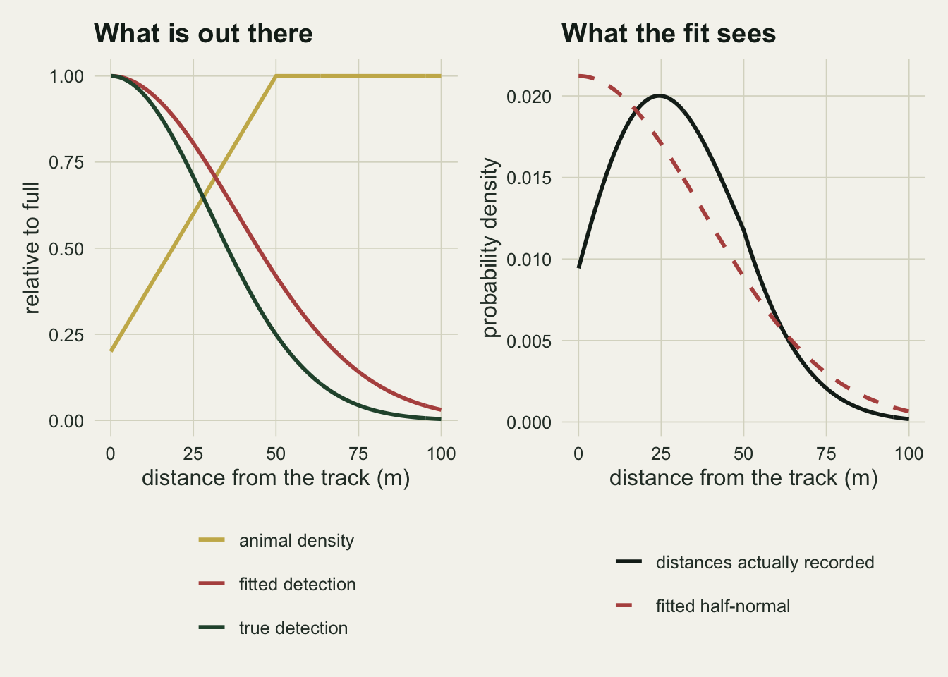
The left panel of the figure is the world and the right panel is the data. The recorded distances are the product of density and detection, rescaled to integrate to one, and that product rises away from the track before it falls. A half-normal cannot rise. The best it can do is spread out: it takes the missing animals near the track and the relatively plentiful ones at 30 to 50 m as a detection function that falls more slowly than it really does. A wider fitted detection function means a wider effective strip, and the same count divided by a wider strip is a lower density.
Nothing in the fit can separate the two curves on the left. The distances identify only their product, so any density profile combined with a matching detection function gives the same likelihood. The estimator resolves the ambiguity by assumption: it sets the density profile flat and hands the whole shape to detection.
How much density the fit loses
The same limiting calculation runs over the whole grid, and it separates two losses. The ratio against the strip density is the fitting error alone. The ratio against the off-track density adds the fact that the covered strip is sparser than the block.
ratio_long <- rbind(
  data.frame(l = lim_tab$l, a = lim_tab$a, ratio = lim_tab$off,
             truth = "against off-track density"),
  data.frame(l = lim_tab$l, a = lim_tab$a, ratio = lim_tab$strip,
             truth = "against density in the strip"))
ratio_long$a_lab <- sprintf("track density %.1f of full", ratio_long$a)
ggplot(ratio_long, aes(l, ratio, colour = a_lab, linetype = truth)) +
  geom_hline(yintercept = 1, colour = te_body, linewidth = 0.5) +
  geom_line(linewidth = 0.9) +
  geom_point(size = 2) +
  scale_colour_manual(values = c(te_rust, te_forest), name = NULL) +
  scale_linetype_manual(values = c("solid", "dashed"), name = NULL) +
  scale_x_continuous(breaks = l_grid) +
  scale_y_continuous(limits = c(0, 1.05)) +
  labs(x = "width of the avoidance gradient (m)",
       y = "estimated / true density",
       title = "The wider the gradient, the more goes missing",
       subtitle = "limiting half-normal fit; half-normal detection with scale 30 m") +
  guides(colour = guide_legend(nrow = 2), linetype = guide_legend(nrow = 2)) +
  theme_datasheet() + theme(legend.position = "bottom")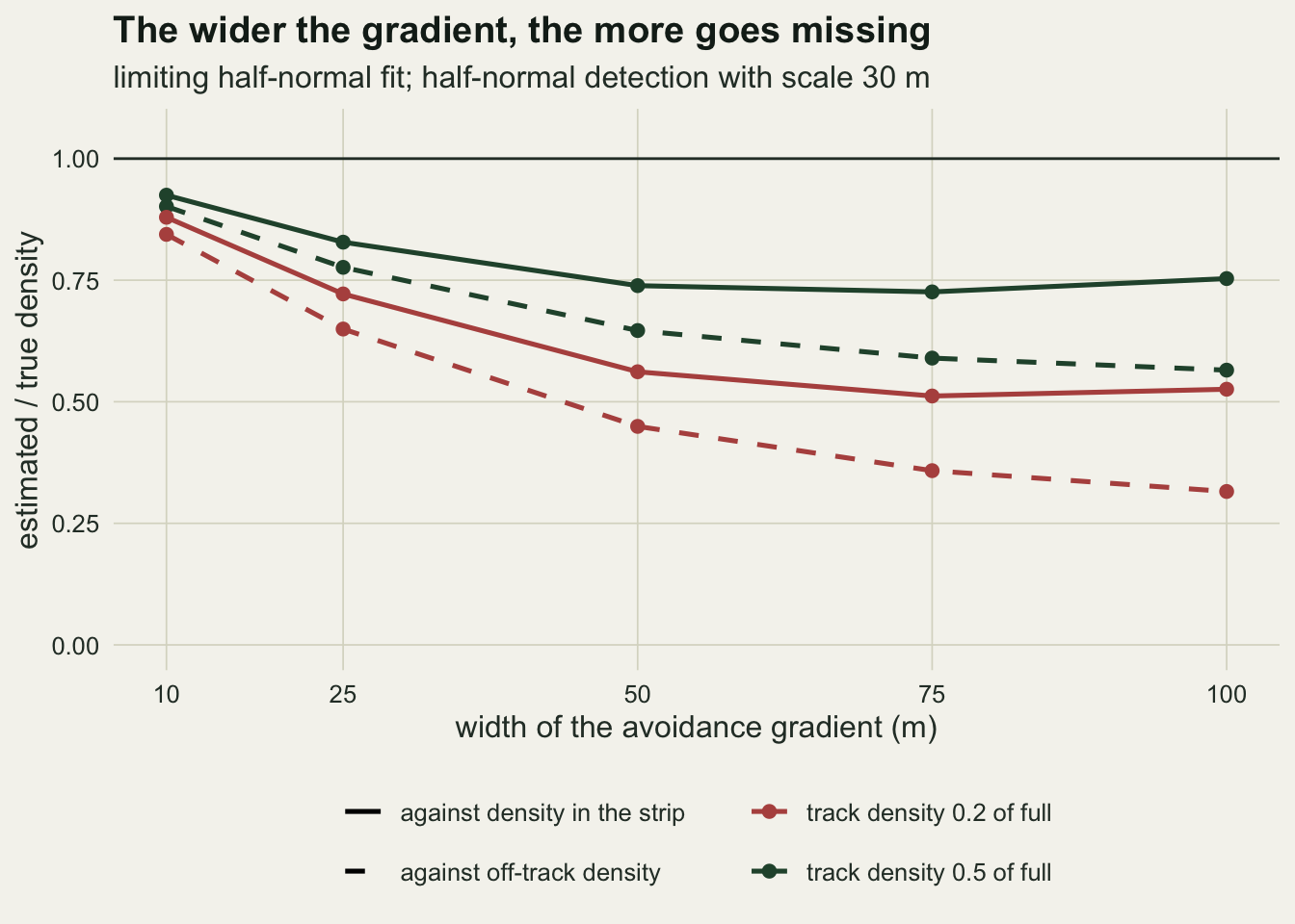
At a track density of one fifth the ratio against the off-track density falls from 0.844 for a 10 m gradient to 0.315 for a 100 m one. The ratio against the strip density changes little beyond 50 m: it is 0.562 at 50 m and 0.526 at 100 m. Once the gradient is wider than the zone where most detections happen, the fit cannot lose much more of the strip, but the strip itself keeps getting less representative of the block, and the off-track ratio carries that. At a track density of one half the off-track ratio runs from 0.902 to 0.565.
A reasonable objection is that the half-normal is the wrong key to test. The hazard-rate key has a shoulder, and a shoulder might follow the flat top of the product better. The limiting hazard-rate fit is computed below by minimising the cross-entropy between the true distance density and the hazard-rate density on a fine grid, which is what maximum likelihood converges to.
x_q  <- seq(0, w_trunc, length.out = 4001)
h_q  <- diff(x_q)[1]
trap <- function(v) h_q * (sum(v) - (v[1] + v[length(v)]) / 2)
g_hr <- function(x, s, b) 1 - exp(-(pmax(x, 1e-9) / s)^(-b))
hr_limit <- function(a_trk, l_grad) {
  f_true <- ramp(x_q, a_trk, l_grad) * g_hn(x_q, sig_true)
  prod_int <- trap(f_true)
  f_true <- f_true / prod_int
  cross_ent <- function(par) {
    g_v <- g_hr(x_q, exp(par[1]), exp(par[2]))
    -trap(f_true * log(pmax(g_v, 1e-300))) + log(trap(g_v))
  }
  opt <- optim(c(log(sig_true), log(3)), cross_ent, control = list(reltol = 1e-12))
  mu_hr <- trap(g_hr(x_q, exp(opt$par[1]), exp(opt$par[2])))
  pbar  <- trap(ramp(x_q, a_trk, l_grad)) / w_trunc
  c(a = a_trk, l = l_grad, off = prod_int / mu_hr, strip = prod_int / mu_hr / pbar,
    shape = exp(opt$par[2]))
}
hr_tab <- as.data.frame(t(mapply(hr_limit, rep(a_grid, each = length(l_grid)),
                                 rep(l_grid, length(a_grid)))))
hr_main <- hr_tab[hr_tab$a == a_main & hr_tab$l == l_main, ]
hr_unif <- hr_limit(1, l_main)
hr_rel_main <- hr_main$off / hr_unif[["off"]]
The hazard-rate key is already wrong without any gradient: fitted to plain half-normal distances it returns 0.877 of the true density, because its shoulder is not the half-normal’s. In the main case it returns 0.362 of the off-track density, which is 0.413 of its own no-gradient value, against 0.449 for the half-normal. The shoulder does not rescue the estimate. A flatter top lets the key absorb even more of the missing animals near the track into a wide detection function, with a fitted shape of 5.8.
Calibrating the test before asking it anything
The goodness-of-fit question needs simulated surveys. Distances are drawn by thinning uniform positions with the product of density and detection, 80 kept per survey, and the Kolmogorov-Smirnov distance is computed against the fitted truncated half-normal for all surveys at once.
draw_prof <- function(n_rep, n_obs, a_trk, l_grad) {
  acc_rate <- integrate(function(x) ramp(x, a_trk, l_grad) * g_hn(x, sig_true),
                        0, w_trunc)$value / w_trunc
  k_draw <- ceiling((n_obs + 8 * sqrt(n_obs) + 20) / acc_rate)
  x_all  <- matrix(runif(n_rep * k_draw, 0, w_trunc), n_rep)
  keep   <- matrix(runif(n_rep * k_draw), n_rep) <
            ramp(x_all, a_trk, l_grad) * g_hn(x_all, sig_true)
  keep   <- keep & (t(apply(keep, 1, cumsum)) <= n_obs)
  stopifnot(all(rowSums(keep) == n_obs))
  matrix(t(x_all)[t(keep)], n_rep, byrow = TRUE)
}
draw_hn <- function(n_rep, n_obs, s) {
  matrix(s * qnorm(0.5 + runif(n_rep * n_obs) * (pnorm(w_trunc / s) - 0.5)), n_rep)
}
ks_root_n <- function(x_mat, s) {
  n_obs <- ncol(x_mat)
  x_srt <- t(apply(x_mat, 1, sort))
  s_mat <- matrix(s, nrow(x_mat), n_obs)
  cdf   <- (pnorm(x_srt / s_mat) - 0.5) / (pnorm(w_trunc / s_mat) - 0.5)
  i_mat <- matrix(seq_len(n_obs), nrow(x_mat), n_obs, byrow = TRUE)
  sqrt(n_obs) * apply(pmax(i_mat / n_obs - cdf, cdf - (i_mat - 1) / n_obs), 1, max)
}
The test statistic has a calibration problem before any gradient enters. The usual p-value from ks.test() assumes the scale was known, but it was fitted to the same distances, and a curve fitted to the data sits closer to them than the truth does. Lilliefors (1967) tabulated the correction for the normal with estimated mean and variance. That table does not apply here, and neither does a single pooled null, because a half-normal truncated at a fixed distance is not a pure scale family: the shape of the truncated curve depends on how the scale compares with the truncation distance. The chunk below simulates the five per cent point of the root-n distance under a true truncated half-normal at ten scales and three sample sizes, with the scale estimated each time, and interpolates at each survey’s fitted scale.
n_levels <- c(80, 300, 1500)
s_cal    <- c(15, 20, 25, 30, 35, 40, 50, 65, 85, 120)
cal_reps <- c(6000, 3000, 800)

set.seed(5190)
crit_tab <- sapply(seq_along(n_levels), function(j) {
  vapply(s_cal, function(s) {
    x_null <- draw_hn(cal_reps[j], n_levels[j], s)
    unname(quantile(ks_root_n(x_null, fit_sig(rowMeans(x_null^2))), 0.95))
  }, 0)
})
crit_at <- function(s, n_obs) {
  approx(s_cal, crit_tab[, match(n_obs, n_levels)], xout = s, rule = 2)$y
}
crit_fixed  <- 1.358   # asymptotic 5 per cent point with the parameter known
crit_lo     <- min(crit_tab[, 1])
crit_hi     <- max(crit_tab[, 1])
crit_30     <- crit_tab[s_cal == sig_true, 1]
reps_main   <- 1000
mc_se_rate  <- sqrt(0.25 / reps_main)
At 80 detections the calibrated five per cent point is 1.124 at the true scale, and across the ten scales it ranges from 1.014 to 1.138, all well below the known-parameter value of 1.358. Read against the known-parameter table, the distance with a fitted scale gives a conservative test, and how conservative depends on the scale.
The grid below runs 1000 surveys of 80 detections in each cell, a number fixed so that the Monte Carlo standard error of any rejection rate is at most 0.016. A cell with no gradient is the null check.
run_cell <- function(n_rep, n_obs, a_trk, l_grad) {
  x_mat  <- draw_prof(n_rep, n_obs, a_trk, l_grad)
  s_hat  <- fit_sig(rowMeans(x_mat^2))
  d_stat <- ks_root_n(x_mat, s_hat)
  lim    <- limit_fit(a_trk, l_grad)
  prod_int  <- lim["off"] * mu_hn(lim["sig"])
  ratio_off <- prod_int / mu_hn(s_hat)
  p_nom <- vapply(seq_len(n_rep), function(i) {
    s_i <- s_hat[i]
    ks.test(x_mat[i, ], function(q) (pnorm(q / s_i) - 0.5) / (pnorm(w_trunc / s_i) - 0.5))$p.value
  }, 0)
  c(n = n_obs, a = a_trk, l = l_grad,
    off = mean(ratio_off), off_se = sd(ratio_off) / sqrt(n_rep),
    strip = mean(ratio_off) / lim[["pbar"]],
    lim_off = lim[["off"]], lim_strip = lim[["strip"]],
    rej_cal = mean(d_stat > crit_at(s_hat, n_obs)),
    rej_nom = mean(p_nom < 0.05))
}
set.seed(8841)
null_main <- run_cell(reps_main, n_det, 1, l_main)
grid_main <- as.data.frame(t(mapply(function(a_trk, l_grad) run_cell(reps_main, n_det, a_trk, l_grad),
                                    rep(a_grid, each = length(l_grid)),
                                    rep(l_grid, length(a_grid)))))
null_se    <- sqrt(null_main[["rej_cal"]] * (1 - null_main[["rej_cal"]]) / reps_main)
gm <- function(a_trk, l_grad, col) grid_main[grid_main$a == a_trk & grid_main$l == l_grad, col]
rel_gap_max <- 100 * max(grid_main$off / grid_main$lim_off - 1)
rel_gap_min <- 100 * min(grid_main$off / grid_main$lim_off - 1)
null_nom_se <- sqrt(null_main[["rej_nom"]] * (1 - null_main[["rej_nom"]]) / reps_main)
With no gradient the calibrated test rejects 0.057 of surveys, with a Monte Carlo standard error of 0.007, against the intended 0.05. The uncalibrated ks.test() p-value with the fitted scale rejects 0.017 (standard error 0.004), about a third of its nominal level. Both are carried forward, because the uncalibrated one is what most analyses would report.
The simulated density ratios match the limiting ones: across the grid the mean over surveys sits between 0.3 and 1.0 per cent above the limiting value, and the no-gradient cell gives 1.009. That small upward excess is the finite-sample bias of dividing by an estimated width; at 80 detections it is a rounding error next to the gradient bias, and the integrals tell the same story as the surveys.
The test misses the gradients that cost most
Put the damage on one axis and the chance of detecting it on the other. If the test protected the estimate, the worst gradients would be caught most often.
pd_df <- grid_main
pd_df$a_lab <- sprintf("track density %.1f of full", pd_df$a)
# label placement: above the peak, left of the crowded pair at half density and of the leftmost point
pd_df$lab_dx <- ifelse(pd_df$l == 25, 0, 0.012)
pd_df$lab_dy <- ifelse(pd_df$l == 25, 0.045, -0.035)
pd_df$lab_hj <- ifelse(pd_df$l == 25, 0.5, 0)
crowd_100 <- pd_df$a == 0.5 & pd_df$l == 100
crowd_75  <- pd_df$a == 0.5 & pd_df$l == 75
pd_df$lab_dx[crowd_100] <- -0.015; pd_df$lab_dy[crowd_100] <- 0;     pd_df$lab_hj[crowd_100] <- 1
pd_df$lab_dx[crowd_75]  <- -0.005; pd_df$lab_dy[crowd_75]  <- 0.045; pd_df$lab_hj[crowd_75]  <- 1
rust_100 <- pd_df$a == 0.2 & pd_df$l == 100
pd_df$lab_dx[rust_100] <- -0.015; pd_df$lab_dy[rust_100] <- 0;     pd_df$lab_hj[rust_100] <- 1
ggplot(pd_df, aes(off, rej_cal, colour = a_lab)) +
  geom_hline(yintercept = 0.05, linetype = "dashed", colour = te_body, linewidth = 0.5) +
  geom_segment(aes(xend = off, y = rej_nom, yend = rej_cal), linewidth = 0.4) +
  geom_path(linewidth = 0.8) +
  geom_point(size = 2.6) +
  geom_point(aes(y = rej_nom), size = 2.2, shape = 21, fill = te_paper) +
  geom_text(aes(x = off + lab_dx, y = rej_cal + lab_dy, label = paste0(l, " m"),
                hjust = lab_hj),
            size = 3.3, show.legend = FALSE) +
  scale_colour_manual(values = c(te_rust, te_forest), name = NULL) +
  scale_x_continuous(limits = c(0.25, 1)) +
  scale_y_continuous(limits = c(0, 0.85)) +
  labs(x = "estimated / off-track density (lower is worse)",
       y = "rejection rate, 80 detections",
       title = "Power does not follow the damage",
       subtitle = "filled: calibrated test; open: ks.test p-value with the fitted scale") +
  theme_datasheet() + theme(legend.position = "bottom")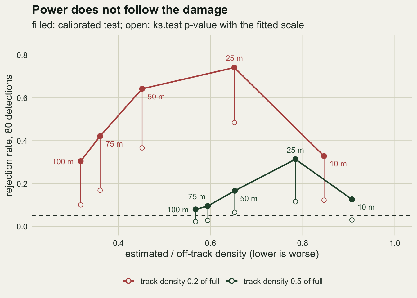
The figure runs the other way. At a track density of one fifth the calibrated test catches the 25 m gradient in 74 per cent of surveys, where the estimate is 0.652 of the off-track density. It catches the 100 m gradient in 30 per cent, where the estimate is 0.318. The uncalibrated p-value that an analyst would actually read rejects those two in 48 and 10 per cent. At a track density of one half the calibrated rates for gradients of 50 m and wider are 0.166, 0.095 and 0.079, and the uncalibrated ones are 0.065, 0.028 and 0.022, while the estimate loses between 35 and 43 per cent of the off-track density.
The shape of the curve has a reason that the limiting fit already contains. Kolmogorov-Smirnov power depends on the largest gap between the distribution of recorded distances and the best half-normal, and that gap can be computed exactly from the same integrals. At a track density of one fifth it is 0.077 for the 10 m gradient, 0.113 for 25 m, 0.096 for 50 m and 0.061 for 100 m. Multiplied by the square root of 80, the 25 m gap is 1.01 and the 100 m gap 0.54, to set against a critical value near 1.12. A narrow gradient takes few animals out of the strip, so the distances barely move. A wide gradient takes many out, but it rises slowly across the whole zone where detection is high, and a wider half-normal absorbs most of it. The departure the test can see is largest in between. Among gradients of 25 m and wider, each step that makes the estimate worse makes the test less likely to object.
More detections, and the test wakes up
Power in a goodness-of-fit test is a function of sample size, and the density bias is not. The same gradients at a track density of one fifth were run again with 300 and 1500 detections per survey, the sort of totals that come from pooling a season of transects or a multi-year programme.
reps_n <- c(400, 150)
set.seed(3306)
grid_more <- do.call(rbind, lapply(1:2, function(j) {
  as.data.frame(t(vapply(c(0, l_grid), function(l_grad) {
    out <- run_cell(reps_n[j], n_levels[j + 1], if (l_grad == 0) 1 else a_main,
                    max(l_grad, 10))
    out[["l"]] <- l_grad
    out
  }, numeric(10))))
}))
base_80 <- rbind(null_main, grid_main[grid_main$a == a_main, ])
base_80$l[1] <- 0
grid_n <- rbind(base_80, grid_more)
pick_n <- function(n_obs, l_grad, col) grid_n[grid_n$n == n_obs & grid_n$l == l_grad, col]
null_reps <- c(reps_main, reps_n)
null_z <- (grid_n$rej_cal[grid_n$l == 0] - 0.05) / sqrt(0.05 * 0.95 / null_reps)
With no gradient the calibrated test rejects 0.055 at 300 detections and 0.053 at 1500, so the calibration holds at the larger sizes, within Monte Carlo error of 0.018 for the smaller replication at 1500.
pn_df <- grid_n
pn_df$n_lab <- factor(sprintf("%d detections", pn_df$n),
                      levels = sprintf("%d detections", n_levels))
ggplot(pn_df, aes(l, rej_cal, colour = n_lab)) +
  geom_hline(yintercept = 0.05, linetype = "dashed", colour = te_body, linewidth = 0.5) +
  geom_line(linewidth = 0.9) +
  geom_point(size = 2.2) +
  scale_colour_manual(values = c(te_gold, te_forest, te_ink), name = NULL) +
  scale_x_continuous(breaks = c(0, l_grid),
                     labels = c("none", as.character(l_grid))) +
  scale_y_continuous(limits = c(0, 1)) +
  labs(x = "width of the avoidance gradient (m)",
       y = "calibrated rejection rate",
       title = "Power follows the sample, not the damage",
       subtitle = "density on the track one fifth of full; dashed line: five per cent") +
  theme_datasheet() + theme(legend.position = "bottom")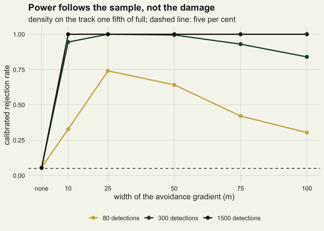
At 300 detections the calibrated test catches the 100 m gradient in 84 per cent of surveys and the uncalibrated p-value in 62 per cent. At 1500 detections the lowest calibrated rejection rate across the five gradients is 1.000. The estimate does not improve with the sample: at 1500 detections the 100 m gradient still returns 0.316 of the off-track density, against 0.318 at 80.
So a passing test on a single season’s track survey says little about the gradient, and a failing test on a pooled data set says only that the data set is large. Neither reading measures the thing that matters, which is how far density at the track differs from density away from it.
What to report
State where the lines were, in relation to tracks, roads, rides and paths, in the methods and not only in the site description. A survey on tracks estimates the density of animals in the strip beside the tracks as seen through a detection function that has absorbed their avoidance; it does not estimate the density of the block, and the main case above, with one fifth of the density on the track recovering over 50 m, puts the loss at 55 per cent of the off-track density.
Show the histogram of perpendicular distances with fine bins near zero, and say whether it rises before it falls. A rise over the first few tens of metres is direct evidence that density or detection is not what the key function assumes. Its absence is not evidence of uniformity: the wide gradients that cost most move the distribution of distances least.
If a goodness-of-fit test is reported, calibrate it for the fitted parameter and the truncation, by parametric bootstrap or a simulated table like the one above, and give the number of detections next to the p-value. The uncalibrated ks.test() p-value with a fitted scale rejected well under its nominal rate here, and at a few hundred detections even a calibrated rejection is mostly telling you the sample size.
The repair is in the design and needs information the distances do not contain. Lines placed at random, or systematically with a random start, make uniformity true by construction. Where tracks must be used, a sample of lines placed away from the tracks, or a measured density profile across the track margin from a separate survey, gives the gradient its own data; the detection function can then be fitted with that profile built in, which is the only way to separate the two curves in the first figure.
Honest limits
The density profile is a straight ramp from the track to full density, with no attraction. Some species use track verges, forage on the flush of grass along rides or travel along the track itself; that gradient runs the other way, piles detections near zero, and makes the half-normal too narrow and the density too high. Nothing above measures that case, and whether a test sees a pile-up at zero more readily than a deficit was not measured.
Detection is one half-normal with a scale of 30 m and a truncation of 100 m. The damage depends on the gradient width relative to the detection scale, so a species detected over 200 m with an avoidance zone of 50 m is closer to the narrow cases here, and one detected over 20 m in dense cover is closer to the wide ones. The grid covers that ratio from a third to a little over three, at two track densities.
The number of detections was held at its expectation in every survey. A real survey has a Poisson or overdispersed count, which adds variance to the density estimate but does not change the ratios, since the gradient bias sits in the fitted width.
The calibrated test uses a table of simulated five per cent points at ten scales and interpolates at the fitted scale, which is an approximation to a parametric bootstrap for each survey. Its null rejection rates came out between 0.053 and 0.057, and the furthest from 0.05 is 1.02 Monte Carlo standard errors away, a gap chance alone produces often. The binned chi-square test that the checking post used was not run, and its power against these gradients is not known from this post.
The hazard-rate result is a limiting calculation, not a simulation with model selection. In practice an analyst would compare keys by AIC, and at 80 detections the choice would vary from survey to survey. The limiting fits say only that neither key, chosen or not, removes the loss.
The track itself was treated as a line of zero width with animals possible right up to it, and observers were assumed to detect animals at their positions before any response to the observer. Responsive movement away from an approaching observer produces a gradient in the recorded positions that looks like the ones simulated here, but it is a different process: it depends on the observer and not on the track, and random line placement does not remove it.
References
Buckland ST, Anderson DR, Burnham KP, Laake JL, Borchers DL, Thomas L 2001 Introduction to Distance Sampling: Estimating Abundance of Biological Populations (ISBN 978-0-19-850927-1)
Lilliefors HW 1967 Journal of the American Statistical Association 62(318):399-402 (10.1080/01621459.1967.10482916)