---
title: "Latent variables in an SEM, from scratch in R"
description: "Soil fertility is not measured, three imperfect indicators are. A one-factor model recovers the slope that every composite of them gets wrong, in base R."
date: "2026-08-06 13:00"
categories: [R, structural equation models, measurement error, ecology tutorial]
image: thumbnail.png
image-alt: "Two lines against a dashed horizontal line marking the true slope, plotted as indicator quality improves: the composite estimate rises steeply from well below the line, crosses it and stays above, peaking before the last point and easing back slightly, while the latent estimate stays close to the line throughout, with one bump at the second loading value."
---
The path analysis on this site works with measured columns: a slope from soil nitrogen to biomass is a slope between two things a machine reported. The reason ecologists reach for a structural equation model is usually the other case. "Soil fertility" is not in the data. "Disturbance" is not in the data. What is in the data is three or four imperfect stand-ins, none of which is the thing, and all of which are correlated because the thing exists.
A one-factor measurement model treats that construct as unobserved and the indicators as noisy expressions of it. The useful part is not the diagram. It is that three indicators contain enough information to estimate how unreliable each of them is, using nothing but their covariances, and to correct the slope accordingly.
## The generator
One latent construct, three indicators of decreasing quality, and one structural slope onto a response.
```{r setup}
#| message: false
#| warning: false
library(ggplot2)

te_paper  <- "#f5f4ee"
te_ink    <- "#16241d"
te_body   <- "#2c3a31"
te_forest <- "#275139"
te_rust   <- "#b5534e"
te_gold   <- "#c9b458"
te_line   <- "#dad9ca"

theme_datasheet <- function() {
  theme_minimal(base_size = 12) +
    theme(plot.background  = element_rect(fill = te_paper, colour = NA),
          panel.background = element_rect(fill = te_paper, colour = NA),
          panel.grid.major = element_line(colour = te_line, linewidth = 0.3),
          panel.grid.minor = element_blank(),
          text             = element_text(colour = te_body),
          plot.title       = element_text(colour = te_ink, face = "bold"),
          axis.text        = element_text(colour = te_body))
}

beta_true <- 0.7

draw_stands <- function(n = 300, load = c(0.6, 0.5, 0.4)) {
  eta <- rnorm(n)                                   # fertility, never observed
  x   <- sapply(load, function(l) l * eta + rnorm(n, 0, sqrt(1 - l^2)))
  colnames(x) <- paste0("x", seq_along(load))
  data.frame(x, y = beta_true * eta + rnorm(n, 0, sqrt(1 - beta_true^2)))
}

set.seed(45)
stands <- draw_stands()
round(cor(stands), 3)
```
The indicators are standardised, so each loading is the correlation between that indicator and the construct, and its square is the share of the indicator's variance that is fertility rather than noise. The best of the three carries `r sprintf("%.0f", 100 * 0.6^2)` per cent signal, the worst `r sprintf("%.0f", 100 * 0.4^2)` per cent.
## One indicator is attenuated, as expected
```{r single}
single <- coef(lm(y ~ x1, data = stands))[["x1"]]
round(c(single_indicator = single, truth = beta_true), 4)
```
The regression on the best single indicator gives `r sprintf("%.3f", single)` against a truth of `r beta_true`. That is ordinary regression dilution and it needs no new theory; the [post on measurement error and regression dilution](../measurement-error-regression-dilution/) derives the attenuation factor and says what it takes to undo it with a reliability estimate from replicates.
The question this post answers is what to do when there are no replicates, but there are several different indicators of the same thing.
## The composite, and why the obvious version is a trap
The instinct is to average the three. It should help, because averaging cancels noise, and it does help, and the way it helps is treacherous.
```{r composite}
raw_comp  <- rowMeans(stands[, c("x1", "x2", "x3")])
std_comp  <- as.numeric(scale(raw_comp))

round(c(raw_composite = coef(lm(stands$y ~ raw_comp))[[2]],
        std_composite = coef(lm(stands$y ~ std_comp))[[2]],
        truth         = beta_true), 4)
```
The raw composite lands on `r sprintf("%.3f", coef(lm(stands$y ~ raw_comp))[[2]])`, which is the number to set against the truth, and it is not pulled down by construction the way the single indicator is, because the two biases in a raw composite work against each other. The standardised composite lands on `r sprintf("%.3f", coef(lm(stands$y ~ std_comp))[[2]])`, well below it. Same numbers, same information, and the version that looks right is the one nobody would report, because a composite on an arbitrary scale is not interpretable and gets standardised before it goes in a table.
The raw version is not right. It is a coincidence, and it is worth seeing the algebra because the coincidence is not stable. Averaging shrinks the scale of the composite by roughly the mean loading, which inflates the slope; the noise in the composite attenuates the slope. With these three loadings the two effects nearly cancel. Change the loadings and they stop cancelling, in either direction.
```{r loading-sweep}
estimators <- function(d) {
  raw <- rowMeans(d[, c("x1", "x2", "x3")])
  c(single = coef(lm(y ~ x1, data = d))[[2]],
    raw    = coef(lm(d$y ~ raw))[[2]],
    std    = coef(lm(d$y ~ as.numeric(scale(raw))))[[2]])
}

sets <- list(weak    = c(0.4, 0.35, 0.3),
             uneven  = c(0.6, 0.5, 0.4),
             strong  = c(0.9, 0.85, 0.8))

set.seed(5)
comp <- t(sapply(sets, function(l)
  rowMeans(replicate(200, estimators(draw_stands(load = l))))))
round(comp, 4)
```
With weak indicators the raw composite reads `r sprintf("%.3f", comp["weak", "raw"])`, below the truth. With strong ones it reads `r sprintf("%.3f", comp["strong", "raw"])`, above it. The middle row is the set used above, and it lands at `r sprintf("%.3f", comp["uneven", "raw"])`: the bias passes through zero somewhere around there, and where it passes depends on the loadings, which are exactly the quantities the analyst does not know. The standardised composite is at least honest about its direction, always attenuated, from `r sprintf("%.3f", comp["weak", "std"])` to `r sprintf("%.3f", comp["strong", "std"])`, but it is still wrong.
An estimator that is unbiased at one configuration and biased in opposite directions on either side of it is not a method. It is a coincidence with a standard error.
## Three indicators identify their own reliability
Here is the part that makes the latent model worth the trouble. Under the one-factor model the covariance between two indicators is the product of their loadings, because the only thing they share is the construct:
```
cov(x1, x2) = lambda1 * lambda2
cov(x1, x3) = lambda1 * lambda3
cov(x2, x3) = lambda2 * lambda3
```
Three equations, three unknowns, and the solution is closed form. Multiply the first two and divide by the third and the other loadings cancel.
```{r closed-form}
S <- cov(stands[, c("x1", "x2", "x3")])
lam1 <- sqrt(S[1, 2] * S[1, 3] / S[2, 3])
lam2 <- S[1, 2] / lam1
lam3 <- S[1, 3] / lam1

round(c(lambda1 = lam1, lambda2 = lam2, lambda3 = lam3,
        truth1 = 0.6, truth2 = 0.5, truth3 = 0.4), 4)
```
The reliabilities were never measured and never assumed. They came out of the pattern of covariances, and the only input was the claim that one common cause explains all three. That claim is what buys the correction, and it is also the whole risk, which the honest limits below return to.
With the loadings in hand the structural slope follows: the covariance between an indicator and the response is that indicator's loading times the slope.
```{r closed-slope}
beta_closed <- cov(stands$x1, stands$y) / lam1
round(c(closed_form = beta_closed, truth = beta_true), 4)
```
## Fitting the whole model at once
The closed form is the right way to see why it works and the wrong way to fit it, because it uses three of the covariances and throws the rest away. The usual estimator fits all four variables together by minimising the discrepancy between the observed covariance matrix and the one the model implies. That is eight parameters against ten distinct covariances, so the model is over-identified by two, and those two spare pieces of information are what a fit statistic would test.
```{r ml-fit}
implied <- function(par) {
  lam <- par[1:3]; th <- exp(par[4:6]); b <- par[7]; ps <- exp(par[8])
  Sg <- matrix(0, 4, 4)
  Sg[1:3, 1:3] <- outer(lam, lam)
  diag(Sg)[1:3] <- lam^2 + th
  Sg[4, 1:3] <- Sg[1:3, 4] <- lam * b
  Sg[4, 4] <- b^2 + ps
  Sg
}

discrepancy <- function(par, Sobs) {
  Sg <- implied(par)
  ev <- eigen(Sg, symmetric = TRUE, only.values = TRUE)$values
  if (min(ev) <= 1e-8) return(1e6)
  sum(diag(Sobs %*% solve(Sg))) + log(det(Sg)) - log(det(Sobs)) - nrow(Sobs)
}

Sobs <- cov(stands)
fit  <- optim(c(0.5, 0.5, 0.5, log(rep(0.5, 3)), 0.5, log(0.5)),
              discrepancy, Sobs = Sobs, method = "BFGS",
              control = list(maxit = 2000))

round(c(lambda1 = fit$par[1], lambda2 = fit$par[2], lambda3 = fit$par[3],
        beta = fit$par[7], truth = beta_true,
        converged = fit$convergence), 4)
```
The fitted structural slope is `r sprintf("%.3f", fit$par[7])` against a truth of `r beta_true`, and the loadings agree with the closed form to within `r sprintf("%.3f", max(abs(fit$par[1:3] - c(lam1, lam2, lam3))))`.
## The four estimators side by side
One data set is one draw. Repeating the whole thing gives the sampling distribution of each approach, and that is what tells you which of them is centred on the answer.
```{r all-four}
fit_beta <- function(d) {
  Sd <- cov(d)
  f <- optim(c(0.5, 0.5, 0.5, log(rep(0.5, 3)), 0.5, log(0.5)),
             discrepancy, Sobs = Sd, method = "BFGS",
             control = list(maxit = 2000))
  f$par[7]
}

set.seed(19)
n_rep <- 200
draws <- lapply(names(sets), function(k) {
  m <- t(replicate(n_rep, {
    d <- draw_stands(load = sets[[k]])
    c(estimators(d), latent = fit_beta(d))
  }))
  data.frame(set = k, m)
})
names(draws) <- names(sets)

round(t(sapply(draws, function(z) colMeans(z[, -1]))), 4)
round(t(sapply(draws, function(z) apply(z[, -1], 2, sd))), 4)
```
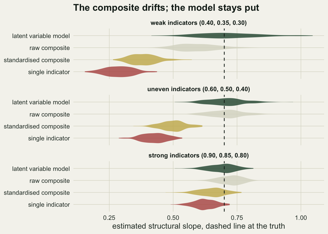
Take the middle row first, the loading set used throughout. Over `r n_rep` data sets the single indicator averages `r sprintf("%.3f", mean(draws$uneven$single))`, the standardised composite `r sprintf("%.3f", mean(draws$uneven$std))`, the raw composite `r sprintf("%.3f", mean(draws$uneven$raw))`, and the latent model `r sprintf("%.3f", mean(draws$uneven$latent))` against a truth of `r beta_true`.
Then read down the raw column. It goes `r sprintf("%.3f", mean(draws$weak$raw))`, `r sprintf("%.3f", mean(draws$uneven$raw))`, `r sprintf("%.3f", mean(draws$strong$raw))` as the indicators improve, sliding straight past the truth, while the latent column stays at `r sprintf("%.3f", mean(draws$weak$latent))`, `r sprintf("%.3f", mean(draws$uneven$latent))`, `r sprintf("%.3f", mean(draws$strong$latent))`. That is the difference between an estimator and a coincidence.
The correction is not free. On the middle set the latent estimate has a standard deviation of `r sprintf("%.3f", sd(draws$uneven$latent))` against `r sprintf("%.3f", sd(draws$uneven$std))` for the standardised composite, so it trades precision for being centred in the right place.
```{r fig-estimators}
#| fig-cap: "Sampling distributions of four estimates of the same structural slope, at three indicator-quality settings, against the true value of 0.7. 200 simulated data sets per panel."
#| fig-alt: "Three stacked panels, one per indicator-quality setting, each with four horizontal violins and a dashed vertical line at the true slope. The single-indicator and standardised-composite violins sit left of the line in every panel and move rightwards as the indicators improve. The raw-composite violin starts left of the line, crosses it in the middle panel and ends right of it. The latent violin is centred on the line in all three panels and is the widest of the four."
long <- do.call(rbind, lapply(names(draws), function(k) {
  z <- draws[[k]]
  do.call(rbind, lapply(c("single", "std", "raw", "latent"), function(e)
    data.frame(set = k, estimator = e, value = z[[e]])))
}))
long$estimator <- factor(long$estimator,
                         levels = c("single", "std", "raw", "latent"),
                         labels = c("single indicator",
                                    "standardised composite",
                                    "raw composite",
                                    "latent variable model"))
long$set <- factor(long$set, levels = names(sets),
                   labels = c("weak indicators (0.40, 0.35, 0.30)",
                              "uneven indicators (0.60, 0.50, 0.40)",
                              "strong indicators (0.90, 0.85, 0.80)"))

ggplot(long, aes(x = value, y = estimator, fill = estimator)) +
  geom_violin(colour = NA, alpha = 0.8, width = 0.95) +
  geom_vline(xintercept = beta_true, linetype = "dashed", colour = te_ink) +
  facet_wrap(~ set, ncol = 1) +
  scale_fill_manual(values = c("single indicator" = te_rust,
                               "standardised composite" = te_gold,
                               "raw composite" = te_line,
                               "latent variable model" = te_forest)) +
  labs(x = "estimated structural slope, dashed line at the truth", y = NULL,
       title = "The composite drifts; the model stays put") +
  theme_datasheet() +
  theme(legend.position = "none",
        strip.text = element_text(colour = te_ink, face = "bold"))
```
## What it costs when the assumption fails
The identification rests on one claim: the indicator errors are uncorrelated, so everything the indicators share is the construct. If two of them share anything else, a common instrument, a common observer, a common season, the model will read that shared nuisance as more construct and adjust accordingly.
```{r correlated-errors}
draw_correlated <- function(n = 300, rho = 0.3, load = c(0.6, 0.5, 0.4)) {
  eta <- rnorm(n)
  shared <- rnorm(n)                       # a second thing x1 and x2 share
  e1 <- sqrt(1 - load[1]^2) * (sqrt(rho) * shared + sqrt(1 - rho) * rnorm(n))
  e2 <- sqrt(1 - load[2]^2) * (sqrt(rho) * shared + sqrt(1 - rho) * rnorm(n))
  e3 <- rnorm(n, 0, sqrt(1 - load[3]^2))
  data.frame(x1 = load[1] * eta + e1,
             x2 = load[2] * eta + e2,
             x3 = load[3] * eta + e3,
             y  = beta_true * eta + rnorm(n, 0, sqrt(1 - beta_true^2)))
}

set.seed(23)
bad <- t(replicate(200, {
  d  <- draw_correlated()
  Sd <- cov(d)
  f  <- optim(c(0.5, 0.5, 0.5, log(rep(0.5, 3)), 0.5, log(0.5)),
              discrepancy, Sobs = Sd, method = "BFGS",
              control = list(maxit = 2000))
  c(latent = f$par[7], std = estimators(d)[["std"]],
    chisq = (nrow(d) - 1) * f$value)
}))
round(c(latent = mean(bad[, "latent"]), std = mean(bad[, "std"]),
        truth = beta_true,
        rejected = mean(bad[, "chisq"] > qchisq(0.95, df = 2))), 4)
```
A correlation of 0.3 between two of the three indicator errors moves the latent estimate to `r sprintf("%.3f", mean(bad[, "latent"]))`. The model reads the shared nuisance as more construct: the loadings on the two contaminated indicators come out above their true values, and the slope shrinks to compensate. The output is not silent about it. The two degrees of freedom the response variable buys give the chi-square some grip here, and it rejects in `r sprintf("%.0f", 100 * mean(bad[, "chisq"] > qchisq(0.95, df = 2)))` per cent of these runs, against the five per cent a correctly specified model would give. What it does not do is say which pair of errors is correlated, and at smaller samples it mostly says nothing at all.
## Honest limits
Three indicators is the minimum, and at the minimum the measurement model is exactly identified, so it cannot be tested. The over-identification above comes from the response variable, not from the indicators. Adding a fourth indicator is the cheapest thing an ecologist can do about that, because it makes the measurement model testable on its own, and it is usually cheaper than another season of fieldwork.
Correlated indicator errors are the failure that matters, and they are only partly visible from these data. Those two degrees of freedom give a chi-square some power against them, as the run above shows, and the power grows with the sample and with the size of the contamination. It is not power an ecological data set can lean on: the same test says almost nothing at the sample sizes most field studies reach, and it never names the pair of errors that is correlated. So the real defences are design defences: measure the indicators with different instruments, different observers or on different occasions, and say in the paper which of those you did.
This post reports no fit indices next to the fitted models, which is not the same as saying a fit statistic carries nothing: the rejection rate in the last section is one doing its job on two degrees of freedom. The conventional cutoffs placed on the derived indices are a different matter, and they are the least defensible part of the method. The [post on checking a structural equation model](../checking-a-structural-equation-model/) covers what a global fit statistic can and cannot certify.
Everything here is standardised and linear, and the loadings are positive. Indicators on genuinely different scales change the arithmetic but not the argument, provided the model is fitted to the covariance matrix rather than the correlation matrix, which matters more than it sounds: standard errors computed from a correlation matrix as if it were a covariance matrix are wrong.
Finally, the correction identifies the slope between the construct and the response. It does not identify what the construct is. Three soil measurements sharing a common cause tell you that a common cause exists and how strongly each indicator reflects it; calling that cause "fertility" is an act of interpretation, and the data are equally happy if it is drainage.
## References
Spearman C 1904 The American Journal of Psychology 15(1):72-101 (10.2307/1412159)
Grace JB, Bollen KA 2008 Environmental and Ecological Statistics 15(2):191-213 (10.1007/s10651-007-0047-7)
Bollen KA 1989 Structural Equations with Latent Variables, Wiley, ISBN 978-0-471-01171-2
## Related tutorials
- [Measurement error and regression dilution](../measurement-error-regression-dilution/)
- [Checking measurement error corrections](../checking-measurement-error-corrections/)
- [Path analysis: direct and indirect effects](../path-analysis-direct-indirect-effects/)
- [Checking a structural equation model](../checking-a-structural-equation-model/)