library(ggplot2)

te_paper  <- "#f5f4ee"
te_ink    <- "#16241d"
te_body   <- "#2c3a31"
te_forest <- "#275139"
te_rust   <- "#b5534e"
te_gold   <- "#c9b458"
te_line   <- "#dad9ca"

theme_datasheet <- function() {
  theme_minimal(base_size = 12) +
    theme(plot.background  = element_rect(fill = te_paper, colour = NA),
          panel.background = element_rect(fill = te_paper, colour = NA),
          panel.grid.major = element_line(colour = te_line, linewidth = 0.3),
          panel.grid.minor = element_blank(),
          text             = element_text(colour = te_body),
          plot.title       = element_text(colour = te_ink, face = "bold"),
          plot.subtitle    = element_text(colour = te_body),
          axis.text        = element_text(colour = te_body))
}Join counts for presence-absence maps
R
spatial statistics
autocorrelation
presence-absence
permutation tests
ecology tutorial
Join counts test clustering on a presence-absence grid. Measuring in R which variance fails, and why a map with few occupied cells needs a permutation test.
A heathland reserve is divided into a grid of 400 one hectare cells, twenty rows by twenty columns, and a survey team walks every cell once in May and records whether a stonechat territory is present. The result is a map of ones and zeros. The question put to it is the obvious one: are the occupied cells bunched together more than chance would bunch them, or are they scattered like a random draw of the same number of cells?
The quickest answer most people reach for is Moran’s I (Moran 1950). The post on spatial autocorrelation and Moran’s I introduces it for a continuous environmental variable on irregular points, with spdep doing the work and a permutation test for the p value. Nothing in the formula stops anyone passing it a vector of zeros and ones, and a piece of advice that is sometimes given says that this is a mistake: that Moran’s I is built for continuous data and that a binary map needs the join count statistics of Moran 1948 instead, because the variance and the reference distribution are wrong for a binary variable.
This post takes that advice apart by measurement. It counts joins on a hand built rook neighbour list in base R, derives the two textbook sets of moments for the count (sampling with and without replacement), checks both against a permutation distribution, and puts Moran’s I on the same maps. Part of the result is the textbook one: Cliff and Ord 1981 already recommend the non free moments when the prevalence comes from the map. The rest is not what the advice predicts. Moran’s I on a binary map behaves almost exactly like the join count, and the variance that does real damage is a join count variance: the free sampling one. The second half of the post shows where every normal approximation fails, which is at low prevalence, and what that failure does to a test.
Two other posts on the site use the same neighbour structure for different jobs. Moran eigenvector spatial filtering turns the adjacency matrix into map patterns and adds them to a GLM, and spatial autocorrelation in occupancy models does the same inside an occupancy likelihood. Both use Moran’s I on model residuals as a diagnostic for continuous residuals; neither asks how to test a raw zero one map, which is the question here.
A grid, its joins and a patchy map
A join is a pair of cells that share an edge. On a rook grid every interior cell has four neighbours, edge cells three and the four corners two. Each join is stored once, as a pair of cell indices, and that list is the whole spatial structure: no weights matrix is ever formed.
side   <- 20
n_cell <- side^2
cell_id <- function(r, cl) (cl - 1) * side + r

# horizontal neighbours within a row, then vertical neighbours within a column
join_from <- c(cell_id(rep(1:side, side - 1), rep(1:(side - 1), each = side)),
               cell_id(rep(1:(side - 1), side), rep(1:side, each = side - 1)))
join_to   <- c(cell_id(rep(1:side, side - 1), rep(2:side, each = side)),
               cell_id(rep(2:side, side), rep(1:side, each = side - 1)))
n_join  <- length(join_from)
deg     <- tabulate(c(join_from, join_to), n_cell)
k_pairs <- sum(deg * (deg - 1) / 2)     # pairs of joins that share a cell
deg_tab <- table(deg)
The grid has 760 joins. The cell degrees split into 4 corners, 72 edge cells and 324 interior cells, and the number of pairs of joins that meet at a common cell is 2164. Those two totals, the join count and the shared cell pair count, are all the moment formulas below need.
To have something to test, maps are generated from a latent surface: independent normal noise smoothed twice by averaging each cell with its rook neighbours, rescaled to unit variance across the cells of each map, and mixed with fresh noise. A mixing weight of zero gives a map with no spatial structure at all, and the example map uses a weight of one half, fixed before anything was run. The cells with the highest latent values are marked occupied, so the number of occupied cells is set exactly.
bb_count <- function(xm) colSums(xm[join_from, , drop = FALSE] * xm[join_to, , drop = FALSE])
bw_count <- function(xm) colSums(xm[join_from, , drop = FALSE] != xm[join_to, , drop = FALSE])

smooth_rook <- function(fm, n_pass) {
  for (i in seq_len(n_pass)) {
    nb_sum <- rowsum(rbind(fm[join_to, , drop = FALSE], fm[join_from, , drop = FALSE]),
                     c(join_from, join_to), reorder = TRUE)
    fm <- (fm + nb_sum) / (1 + deg)
  }
  fm
}

make_maps <- function(n_map, n_occ, w_mix, n_pass = 2) {
  sm <- scale(smooth_rook(matrix(rnorm(n_cell * n_map), n_cell), n_pass))
  fm <- sqrt(w_mix) * sm + sqrt(1 - w_mix) * matrix(rnorm(n_cell * n_map), n_cell)
  apply(fm, 2, function(v) as.numeric(rank(-v, ties.method = "first") <= n_occ))
}

w_example <- 0.5
n_occ     <- 140
set.seed(3071)
map_a <- make_maps(1, n_occ, w_example)
bb_a  <- bb_count(map_a)
bw_a  <- bw_count(map_a)
ww_a  <- n_join - bb_a - bw_a
The example map has 140 occupied cells, a prevalence of 0.35. Among its 760 joins, 128 link two occupied cells (black to black, BB in the old notation), 285 link an occupied cell to an empty one (BW), and 347 link two empty cells (WW). Clustering shows up as too many BB and WW joins and too few BW joins, and the three counts always sum to the total, so only two of them carry information.
cell_xy <- data.frame(cl = rep(1:side, each = side), rw = rep(1:side, side),
                      occ = factor(map_a[, 1], levels = c(0, 1), labels = c("empty", "occupied")))
bb_idx  <- which(map_a[join_from, 1] * map_a[join_to, 1] == 1)
seg_df  <- data.frame(x0 = cell_xy$cl[join_from[bb_idx]], y0 = cell_xy$rw[join_from[bb_idx]],
                      x1 = cell_xy$cl[join_to[bb_idx]],   y1 = cell_xy$rw[join_to[bb_idx]])

ggplot(cell_xy, aes(cl, rw)) +
  geom_tile(aes(fill = occ), colour = te_paper, linewidth = 0.4) +
  geom_segment(data = seg_df, aes(x = x0, y = y0, xend = x1, yend = y1),
               colour = te_rust, linewidth = 0.8) +
  scale_fill_manual(values = c(empty = te_line, occupied = te_forest), name = NULL) +
  coord_equal(expand = FALSE) +
  labs(x = "column", y = "row", title = "A patchy presence map",
       subtitle = "red segments: the BB joins between neighbouring occupied cells") +
  theme_datasheet() +
  theme(legend.position = "bottom", panel.grid.major = element_blank())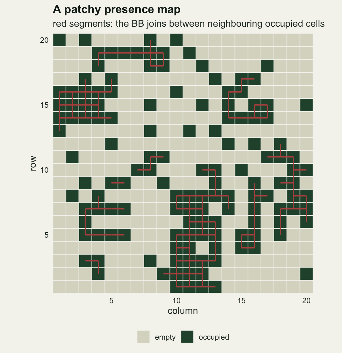
Two sets of moments for one count
The expected BB count is easy: each join is BB with the probability that both of its cells are occupied. The variance needs the covariance between joins, and the grid enters only through how joins overlap. A join paired with itself contributes the probability of two occupied cells; an ordered pair of joins sharing one cell (there are twice the shared pair count of these) contributes the probability of three; every other ordered pair contributes the probability of four.
Those probabilities depend on the sampling model. Under free sampling each cell is occupied independently with probability p, so the probability of k occupied cells is p to the power k. Under non free sampling the number of occupied cells is fixed at the observed value and the occupied cells are a random subset, so the probabilities are falling factorial ratios. Cliff and Ord 1981 give both sets, with the BW moments alongside; the function below writes them out.
join_moments <- function(n_occ, free) {
  n_emp <- n_cell - n_occ
  if (free) {
    p <- n_occ / n_cell; q <- 1 - p
    p_k  <- p^(1:4)
    p_bw <- c(2 * p * q, p * q, 4 * p^2 * q^2)
  } else {
    p_k  <- sapply(1:4, function(k) prod((n_occ - 0:(k - 1)) / (n_cell - 0:(k - 1))))
    p_bw <- c(2 * n_occ * n_emp / (n_cell * (n_cell - 1)),
              (n_occ * n_emp * (n_emp - 1) + n_emp * n_occ * (n_occ - 1)) /
                (n_cell * (n_cell - 1) * (n_cell - 2)),
              4 * n_occ * (n_occ - 1) * n_emp * (n_emp - 1) / prod(n_cell - 0:3))
  }
  n_other <- n_join^2 - n_join - 2 * k_pairs
  e_bb <- n_join * p_k[2]
  v_bb <- n_join * p_k[2] + 2 * k_pairs * p_k[3] + n_other * p_k[4] - e_bb^2
  e_bw <- n_join * p_bw[1]
  v_bw <- n_join * p_bw[1] + 2 * k_pairs * p_bw[2] + n_other * p_bw[3] - e_bw^2
  c(e_bb = e_bb, sd_bb = sqrt(v_bb), e_bw = e_bw, sd_bw = sqrt(v_bw))
}

mom_free <- join_moments(n_occ, free = TRUE)
mom_nonf <- join_moments(n_occ, free = FALSE)
z_bb_free <- (bb_a - mom_free[["e_bb"]]) / mom_free[["sd_bb"]]
z_bb_nonf <- (bb_a - mom_nonf[["e_bb"]]) / mom_nonf[["sd_bb"]]
z_bw_free <- (bw_a - mom_free[["e_bw"]]) / mom_free[["sd_bw"]]
z_bw_nonf <- (bw_a - mom_nonf[["e_bw"]]) / mom_nonf[["sd_bw"]]
sd_ratio  <- mom_free[["sd_bb"]] / mom_nonf[["sd_bb"]]
The two expectations are almost the same: 93.1 BB joins under free sampling and 92.7 under non free sampling. The standard deviations are not. Free sampling gives 14.22 and non free sampling 6.41, a ratio of 2.22. The observed 128 BB joins therefore sit 2.45 standard deviations above expectation by the first yardstick and 5.51 by the second. The BW count tells the same story from the other side, at -3.65 and -4.91.
The size of the gap has a plain reason. Under free sampling the number of occupied cells is itself random, and most of the variance of the BB count is variance in how many occupied cells there are, not in where they sit: the non free variance is only 0.20 of the free one. A map in hand has a known number of occupied cells, and the null hypothesis of interest is about their arrangement, so the conditional, non free moments are the ones that answer the question. A permutation of the observed map is exactly the non free null, which gives a direct check on the algebra, and Moran’s I can be computed from the same permuted maps.
s0 <- 2 * n_join; s1 <- 4 * n_join; s2 <- sum((2 * deg)^2)
e_moran <- -1 / (n_cell - 1)

moran_i <- function(xm) {
  zm <- sweep(xm, 2, colMeans(xm))
  2 * colSums(zm[join_from, , drop = FALSE] * zm[join_to, , drop = FALSE]) *
    (n_cell / s0) / colSums(zm^2)
}
sd_moran_norm <- sqrt((n_cell^2 * s1 - n_cell * s2 + 3 * s0^2) /
                        ((n_cell^2 - 1) * s0^2) - e_moran^2)
sd_moran_rand <- function(n_occ) {
  x0 <- c(rep(1, n_occ), rep(0, n_cell - n_occ)) - n_occ / n_cell
  b2 <- n_cell * sum(x0^4) / sum(x0^2)^2
  nn <- n_cell
  sqrt((nn * ((nn^2 - 3 * nn + 3) * s1 - nn * s2 + 3 * s0^2) -
          b2 * ((nn^2 - nn) * s1 - 2 * nn * s2 + 6 * s0^2)) /
         ((nn - 1) * (nn - 2) * (nn - 3) * s0^2) - e_moran^2)
}

perm_null <- function(n_occ, n_perm, chunk = 5000) {
  bb_out <- numeric(0); i_out <- numeric(0)
  while (length(bb_out) < n_perm) {
    m_now <- min(chunk, n_perm - length(bb_out))
    xm  <- matrix(0, n_cell, m_now)
    pos <- replicate(m_now, sample.int(n_cell, n_occ))
    xm[cbind(as.vector(pos), rep(seq_len(m_now), each = n_occ))] <- 1
    bb_out <- c(bb_out, bb_count(xm)); i_out <- c(i_out, moran_i(xm))
  }
  list(bb = bb_out, moran = i_out)
}
perm_p <- function(obs, null_vals) (1 + sum(null_vals >= obs)) / (1 + length(null_vals))

n_perm <- 40000
set.seed(3072)
null_a <- perm_null(n_occ, n_perm)
perm_mean_bb <- mean(null_a$bb); perm_sd_bb <- sd(null_a$bb)
perm_sd_i    <- sd(null_a$moran)

i_a      <- moran_i(map_a)
z_i_norm <- (i_a - e_moran) / sd_moran_norm
z_i_rand <- (i_a - e_moran) / sd_moran_rand(n_occ)
cor_bb_i <- cor(null_a$bb, null_a$moran)
p_perm_bb_a <- perm_p(bb_a, null_a$bb)
n_above_a   <- sum(null_a$bb >= bb_a)
Across 40000 random rearrangements of the 140 occupied cells, the BB count has a mean of 92.67 and a standard deviation of 6.39, against the non free values of 92.67 and 6.41. The free sampling standard deviation of 14.22 describes a different experiment. 0 of the permutations reached the observed count, so the permutation p value is 0.000025, its floor.
Now Moran’s I on the same zeros and ones. The map gives I = 0.184. Its z score is 5.16 with the variance that assumes normal data and 5.15 with the randomisation variance, which uses the kurtosis of the data; the non free BB z score was 5.51. The permutation standard deviation of I is 0.03606, and the two analytic values are 0.03610 and 0.03617. Across the permuted maps the correlation between I and the BB count is 0.975.
That correlation is algebra, not luck. With a zero one variable the numerator of I expands into twice the BB count, minus a term in the sum of the degrees of the occupied cells, plus a constant. On a torus every degree is four, the middle term is fixed once the number of occupied cells is known, and I is an exact linear function of BB. On a grid with edges the degrees vary, so the two statistics part slightly, because an occupied cell on the boundary has fewer chances to form joins. The advice to avoid Moran’s I on binary data is right that the normality variance was derived for another kind of data, but on this map the three z scores for clustering lie within 0.36 of each other. The number that misleads is the free sampling one.
null_df  <- data.frame(bb = null_a$bb)
bb_grid  <- seq(40, 150, by = 0.5)
curve_df <- rbind(
  data.frame(bb = bb_grid, dens = dnorm(bb_grid, mom_nonf[["e_bb"]], mom_nonf[["sd_bb"]]),
             model = "non free sampling"),
  data.frame(bb = bb_grid, dens = dnorm(bb_grid, mom_free[["e_bb"]], mom_free[["sd_bb"]]),
             model = "free sampling"))

ggplot(null_df, aes(bb)) +
  geom_histogram(aes(y = after_stat(density)), binwidth = 1,
                 fill = te_line, colour = NA) +
  geom_line(data = curve_df, aes(bb, dens, colour = model), linewidth = 0.9) +
  geom_vline(xintercept = bb_a, colour = te_rust, linetype = "dashed", linewidth = 0.8) +
  annotate("text", x = bb_a - 2, y = 0.055, label = "example map", hjust = 1,
           colour = te_rust, size = 3.8) +
  scale_colour_manual(values = c("non free sampling" = te_forest,
                                 "free sampling" = te_gold), name = NULL) +
  labs(x = "BB joins", y = "density",
       title = "The permutation null is the non free one",
       subtitle = "grey: 40000 random arrangements of the same 140 occupied cells") +
  theme_datasheet() +
  theme(legend.position = "bottom")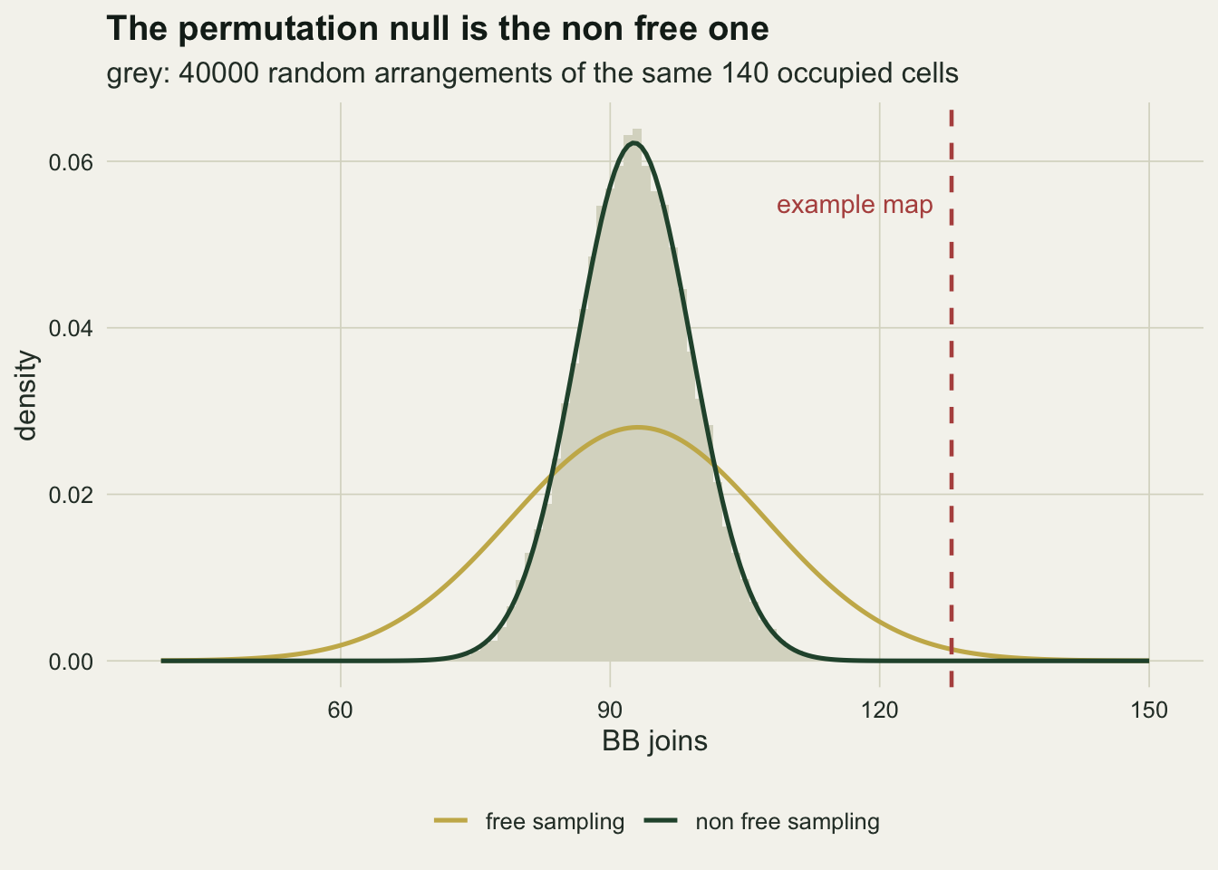
Free sampling with an estimated prevalence
The free sampling formulas are not wrong for their own model. If cells really are occupied independently with a probability known in advance, the free moments are the correct ones. The trouble is that p is never known in advance; it is estimated from the same map, as the fraction of cells occupied. That plug in step is what the next chunk measures, on maps generated exactly under the free sampling model, where no clustering exists and a five per cent test should reject five per cent of the time.
n_bern <- 20000
p_true <- 0.35
z_crit <- qnorm(0.95)
set.seed(3073)
bern_maps <- matrix(rbinom(n_cell * n_bern, 1, p_true), n_cell)
bern_bb   <- bb_count(bern_maps)
bern_occ  <- colSums(bern_maps)

mom_true <- join_moments(n_cell * p_true, free = TRUE)   # uses p_true directly
z_true   <- (bern_bb - mom_true[["e_bb"]]) / mom_true[["sd_bb"]]
mom_hat_free <- t(vapply(bern_occ, join_moments, numeric(4), free = TRUE))
mom_hat_nonf <- t(vapply(bern_occ, join_moments, numeric(4), free = FALSE))
z_hat_free <- (bern_bb - mom_hat_free[, "e_bb"]) / mom_hat_free[, "sd_bb"]
z_hat_nonf <- (bern_bb - mom_hat_nonf[, "e_bb"]) / mom_hat_nonf[, "sd_bb"]

rej_true <- mean(z_true >= z_crit)
rej_free <- mean(z_hat_free >= z_crit)
rej_nonf <- mean(z_hat_nonf >= z_crit)
se_rate  <- function(r, n) sqrt(r * (1 - r) / n)
sd_z_free <- sd(z_hat_free); sd_z_nonf <- sd(z_hat_nonf)
Over 20000 maps with every cell occupied independently at probability 0.35, the one sided test at five per cent rejects in 0.0539 of maps when the true p is used in the free formulas (Monte Carlo standard error 0.0016). Replace the true p with the estimate from each map, which is what anyone analysing a real survey must do, and the rejection rate drops to 0.00010. The non free z score on the same maps rejects in 0.0507, with standard error 0.0016.
The standard deviation of the plug in free z score across these null maps is 0.453, where a calibrated z score should have one; the non free z score has 1.002. Estimating p from the map removes the variation in the number of occupied cells from the count, while the free variance still charges for it. The plug in free test is not slightly conservative; it almost never rejects under the null, and the price shows up as lost power later in the post.
Five per cent prevalence and the normal approximation
Everything so far used a prevalence of 0.35. Scarce species give sparse maps. At twenty occupied cells in four hundred, the expected BB count is under two, and a count that small is a handful of integers with a long right tail. The next chunk builds the exact permutation null for a range of occupied cell numbers and records the true level of each normal approximation test at a nominal five per cent, together with the level the permutation test actually achieves when it must pick an integer cut off.
occ_grid <- c(4, 8, 12, 16, 20, 24, 30, 40, 60, 80, 100, 140, 200)
n_perm_sweep <- 40000
set.seed(3074)
size_tab <- do.call(rbind, lapply(occ_grid, function(k_occ) {
  nl <- perm_null(k_occ, n_perm_sweep)
  mn <- join_moments(k_occ, free = FALSE)
  mf <- join_moments(k_occ, free = TRUE)
  tail_prob <- sapply(0:max(nl$bb), function(v) mean(nl$bb >= v))
  cut_perm  <- which(tail_prob <= 0.05)[1] - 1
  data.frame(n_occ = k_occ,
             bb_nonfree = mean((nl$bb - mn[["e_bb"]]) / mn[["sd_bb"]] >= z_crit),
             bb_free    = mean((nl$bb - mf[["e_bb"]]) / mf[["sd_bb"]] >= z_crit),
             moran_rand = mean((nl$moran - e_moran) / sd_moran_rand(k_occ) >= z_crit),
             moran_norm = mean((nl$moran - e_moran) / sd_moran_norm >= z_crit),
             perm_level = mean(nl$bb >= cut_perm))
}))
se_size <- se_rate(0.05, n_perm_sweep)
row20   <- size_tab[size_tab$n_occ == 20, ]
row8    <- size_tab[size_tab$n_occ == 8, ]
row4    <- size_tab[size_tab$n_occ == 4, ]
row12   <- size_tab[size_tab$n_occ == 12, ]
mom8    <- join_moments(8, free = FALSE)
cut8    <- mom8[["e_bb"]] + z_crit * mom8[["sd_bb"]]
big_occ <- size_tab[size_tab$n_occ >= 60, ]
With 40000 permutations per row, a rate near five per cent carries a Monte Carlo standard error of about 0.0011. At 20 occupied cells, the five per cent prevalence of a scarce species on this grid, the non free BB z test rejects in 0.1009 of random maps, roughly double its nominal level. Moran’s I with the randomisation variance rejects in 0.0824 and with the normality variance in 0.0677. The permutation test at the same nominal level achieves 0.0301, below five per cent because the count is an integer.
The failure is not monotone in prevalence. At 4 occupied cells the normal approximation tests reject in 0.0555 of maps while the permutation test can only achieve 0.0011; at 12 the non free BB test reaches 0.1290. At 8 occupied cells both BB normal tests and the permutation test reject in 0.0273 of maps, because the normal cut off of 1.10 joins falls between the same two integers as the permutation cut off, so the tests are the same test. The level of an approximate test on a discrete statistic jumps as the lattice of possible values slides past the cut off, and the sweep shows a sawtooth rather than a smooth curve. From 60 occupied cells upwards the non free BB test lies between 0.0475 and 0.0578, and the plug in free test is at most 0.0095 throughout that range.
size_long <- rbind(
  data.frame(n_occ = size_tab$n_occ, rate = size_tab$bb_nonfree, test = "BB, non free normal"),
  data.frame(n_occ = size_tab$n_occ, rate = size_tab$moran_rand, test = "Moran I, randomisation"),
  data.frame(n_occ = size_tab$n_occ, rate = size_tab$bb_free,    test = "BB, free normal, p estimated"),
  data.frame(n_occ = size_tab$n_occ, rate = size_tab$perm_level, test = "permutation, achieved level"))
size_long$test <- factor(size_long$test, levels = unique(size_long$test))
size_long$lw <- c(2.2, 1.4, 0.9, 0.5)[as.integer(size_long$test)]   # wider lines drawn first

ggplot(size_long, aes(n_occ, rate, colour = test)) +
  geom_hline(yintercept = 0.05, linetype = "dashed", colour = te_ink, linewidth = 0.5) +
  geom_line(aes(linewidth = lw)) +
  geom_point(size = 2) +
  scale_linewidth_identity() +
  scale_colour_manual(values = c(te_forest, te_gold, te_rust, "grey45"), name = NULL) +
  scale_x_log10(breaks = occ_grid) +
  guides(colour = guide_legend(nrow = 2)) +
  labs(x = "occupied cells (log scale)", y = "rejection rate under the null",
       title = "Sparse maps break the normal approximation",
       subtitle = "dashed: nominal five per cent; coinciding tests show as nested lines") +
  theme_datasheet() +
  theme(legend.position = "bottom")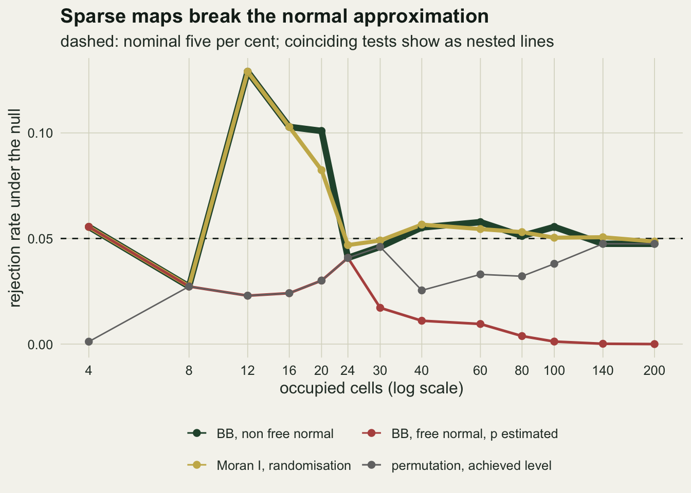
The shape of the null at twenty occupied cells explains the first row of that sweep.
n_low <- 20
set.seed(3075)
null_low <- perm_null(n_low, n_perm)
mom_low  <- join_moments(n_low, free = FALSE)
pmf_low  <- as.data.frame(table(factor(null_low$bb, levels = 0:max(null_low$bb))) / n_perm)
names(pmf_low) <- c("bb", "prob")
pmf_low$bb <- as.numeric(as.character(pmf_low$bb))
cut_norm  <- mom_low[["e_bb"]] + z_crit * mom_low[["sd_bb"]]
p_zero    <- mean(null_low$bb == 0)
skew_low  <- mean((null_low$bb - mean(null_low$bb))^3) / sd(null_low$bb)^3
tail_norm <- mean(null_low$bb >= ceiling(cut_norm))

set.seed(3076)
map_low <- make_maps(1, n_low, w_example)
bb_low  <- bb_count(map_low)
z_low   <- (bb_low - mom_low[["e_bb"]]) / mom_low[["sd_bb"]]
p_norm_low <- pnorm(z_low, lower.tail = FALSE)
p_perm_low <- perm_p(bb_low, null_low$bb)
The expected BB count is 1.81 with a standard deviation of 1.28. A map with no BB joins at all occurs in 0.147 of random arrangements, and the skewness of the null is 0.65. The normal cut off sits at 3.92 joins, so any map with 4 or more BB joins is called significant, and that happens in 0.1035 of random maps.
A single sparse map from the same generator, with the same mixing weight of one half, has 5 BB joins. The normal approximation gives z = 2.49 and a one sided p of 0.0064; the permutation p is 0.0302. One map proves little in either direction, which is why the power comparison below runs over many.
dens_low <- data.frame(bb = seq(-2, 9, by = 0.05))
dens_low$dens <- dnorm(dens_low$bb, mom_low[["e_bb"]], mom_low[["sd_bb"]])

ggplot(pmf_low[pmf_low$bb <= 9, ], aes(bb, prob)) +
  geom_col(fill = te_line, colour = NA, width = 0.8) +
  geom_line(data = dens_low, aes(bb, dens), colour = te_forest, linewidth = 0.9) +
  geom_vline(xintercept = cut_norm, colour = te_rust, linetype = "dashed", linewidth = 0.8) +
  scale_x_continuous(breaks = 0:9) +
  labs(x = "BB joins", y = "probability",
       title = "Twenty occupied cells: a skewed count",
       subtitle = "grey: permutation null; green: normal curve; dashed red: normal cut off") +
  theme_datasheet()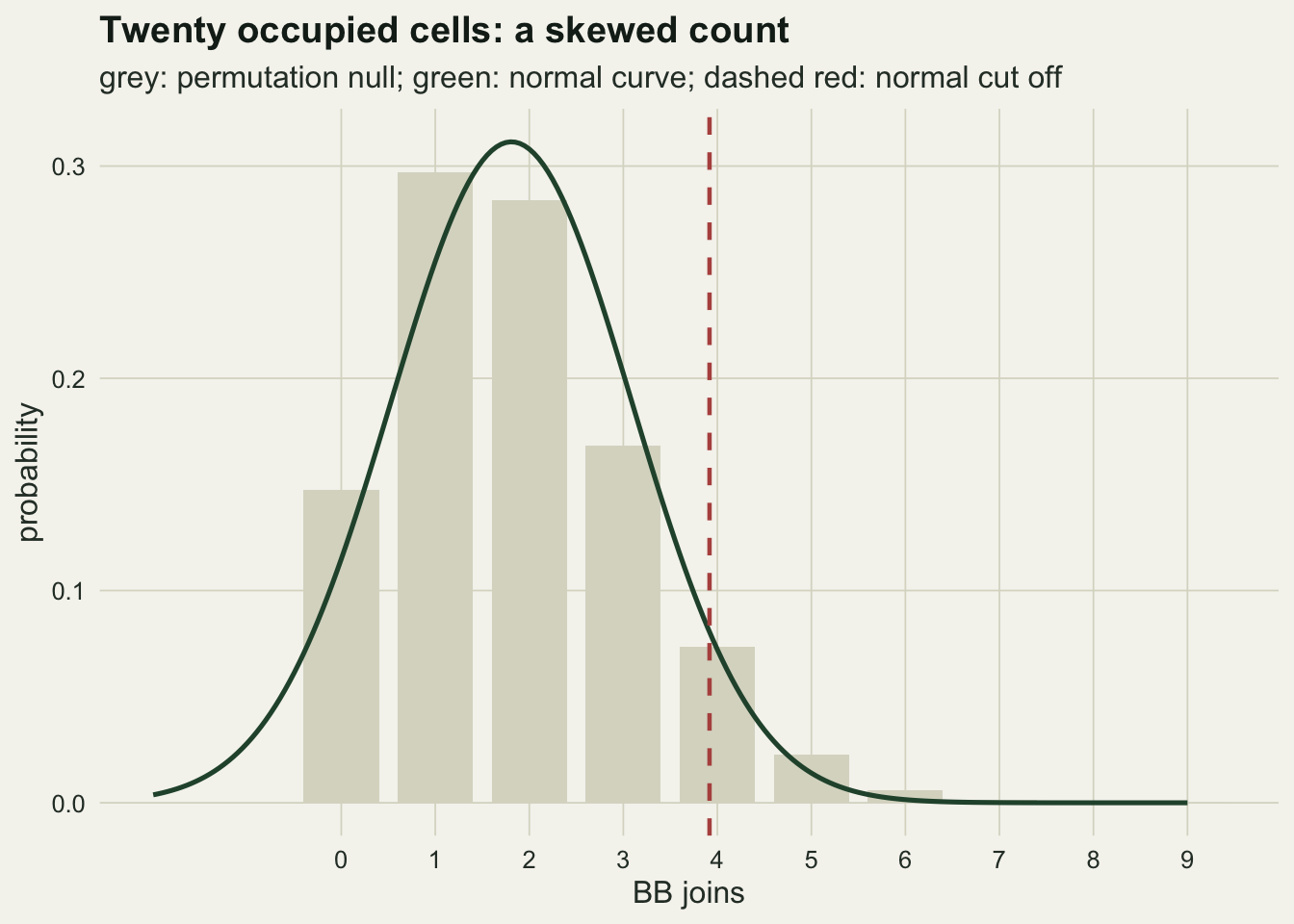
What the choice of test costs in power
Level is half of the comparison. The other half is how often each test finds clustering that is there. The chunk below generates 1000 maps at each of several mixing weights, from zero (no structure) to one half (the example map), at both prevalences, and runs four tests on every map. The permutation p uses the null already built for that number of occupied cells, which is valid because the non free null depends only on the grid and the count.
w_grid <- c(0, 0.05, 0.1, 0.15, 0.2, 0.3, 0.4, 0.5)
n_map  <- 1000
null_140 <- null_a$bb
set.seed(3077)
pow_tab <- do.call(rbind, lapply(c(n_occ, n_low), function(k_occ) {
  null_k <- if (k_occ == n_occ) null_140 else null_low$bb
  srt <- sort(null_k)
  mn <- join_moments(k_occ, free = FALSE); mf <- join_moments(k_occ, free = TRUE)
  sdr <- sd_moran_rand(k_occ)
  do.call(rbind, lapply(w_grid, function(w_now) {
    xm <- make_maps(n_map, k_occ, w_now)
    bb <- bb_count(xm); mi <- moran_i(xm)
    p_perm <- (1 + length(srt) - findInterval(bb, srt, left.open = TRUE)) / (1 + length(srt))
    data.frame(n_occ = k_occ, w_mix = w_now,
               bb_nonfree = mean((bb - mn[["e_bb"]]) / mn[["sd_bb"]] >= z_crit),
               bb_free    = mean((bb - mf[["e_bb"]]) / mf[["sd_bb"]] >= z_crit),
               moran_rand = mean((mi - e_moran) / sdr >= z_crit),
               permutation = mean(p_perm <= 0.05),
               diff_moran_bb = mean((mi - e_moran) / sdr >= z_crit) -
                 mean((bb - mn[["e_bb"]]) / mn[["sd_bb"]] >= z_crit),
               se_diff = sd(((mi - e_moran) / sdr >= z_crit) -
                 ((bb - mn[["e_bb"]]) / mn[["sd_bb"]] >= z_crit)) / sqrt(n_map))
  }))
}))
pw_hi  <- pow_tab[pow_tab$n_occ == n_occ & pow_tab$w_mix == 0.2, ]
pw_lo  <- pow_tab[pow_tab$n_occ == n_low & pow_tab$w_mix == 0.2, ]
pw_lo0 <- pow_tab[pow_tab$n_occ == n_low & pow_tab$w_mix == 0, ]
pw_hi5 <- pow_tab[pow_tab$n_occ == n_occ & pow_tab$w_mix == 0.5, ]
se_pow <- se_rate(0.5, n_map)
mf_low   <- join_moments(n_low, free = TRUE)
cut_free_low <- mf_low[["e_bb"]] + z_crit * mf_low[["sd_bb"]]
cut_perm_low <- which(sapply(0:max(null_low$bb), function(v) mean(null_low$bb >= v)) <= 0.05)[1] - 1
Each rate rests on 1000 maps, so its Monte Carlo standard error is at most 0.016. At 140 occupied cells and a mixing weight of 0.2, the non free BB test detects clustering in 0.656 of maps, the permutation test in 0.656 and Moran’s I in 0.699. The plug in free sampling test detects it in 0.089. Moran’s I is slightly ahead of the BB count here: the paired difference over the same maps is 0.043 with a standard error of 0.009. At the example weight of one half the four rates are 0.998, 0.998, 0.999 and 0.909 in the same order, so even strong clustering leaves the free test behind.
Part of the Moran advantage at 140 cells is level, not sensitivity. Like the permutation test, the BB normal test is a cut off on an integer count, so it cannot sit at exactly five per cent either. The next chunk holds Moran’s I to the level the BB normal test actually achieves on the permutation null, by taking its critical value from the permuted values of I, and compares the two on a fresh set of maps at a weight of 0.2.
n_match <- 4000
set.seed(3078)
xm_match <- make_maps(n_match, n_occ, 0.2)
bb_match <- bb_count(xm_match); mi_match <- moran_i(xm_match)
sdr_140  <- sd_moran_rand(n_occ)
lev_bb_140 <- mean((null_a$bb - mom_nonf[["e_bb"]]) / mom_nonf[["sd_bb"]] >= z_crit)
lev_mi_140 <- mean((null_a$moran - e_moran) / sdr_140 >= z_crit)
srt_i   <- sort(null_a$moran)
tail_i  <- 1 - findInterval(srt_i, srt_i, left.open = TRUE) / length(srt_i)
cut_i   <- srt_i[which(tail_i <= lev_bb_140)[1]]
lev_mi_matched <- mean(null_a$moran >= cut_i)
rej_bb_m  <- (bb_match - mom_nonf[["e_bb"]]) / mom_nonf[["sd_bb"]] >= z_crit
rej_mi_z  <- (mi_match - e_moran) / sdr_140 >= z_crit
rej_mi_lm <- mi_match >= cut_i
gap_raw <- mean(rej_mi_z - rej_bb_m);  se_gap_raw <- sd(rej_mi_z - rej_bb_m) / sqrt(n_match)
gap_lm  <- mean(rej_mi_lm - rej_bb_m); se_gap_lm  <- sd(rej_mi_lm - rej_bb_m) / sqrt(n_match)
On the 40000 permuted maps the BB normal test rejects in 0.0454 and Moran’s I with the randomisation variance in 0.0494. With its critical value moved to match, Moran’s I runs at 0.0454. Over 4000 new maps the BB test detects clustering in 0.655, Moran’s I with its z test in 0.694 and the level matched Moran’s I in 0.682. The paired gap over BB shrinks from 0.038 (standard error 0.004) to 0.027 (standard error 0.004). What is left is a real, small advantage for I at equal level. One plausible reason is the degree term in its numerator, which treats an occupied boundary cell differently from an interior one while the raw count does not; this post does not test that explanation.
At 20 occupied cells the normal approximation tests reject more often, and the reason is their level rather than their sensitivity. With no structure at all the non free BB test already rejects in 0.084 of maps (from 1000 maps, standard error 0.009; the level sweep with 40000 permutations gave 0.1009) and Moran’s I in 0.067, against 0.023 for the permutation test. The non free normal cut off is 3.92 joins, so it rejects from 4 joins, while the permutation test rejects from 5: on this count the normal test is simply the exact test run at a level of 0.1035 on the permutation null. At a weight of 0.2 the rates are 0.322, 0.293 and 0.164. The plug in free test gives 0.164, identical to the permutation test, because its cut off of 4.45 joins also rejects from 5. That agreement is an accident of where the integers fall, as the level sweep showed.
pow_long <- do.call(rbind, lapply(c("bb_nonfree", "moran_rand", "bb_free", "permutation"),
  function(col) data.frame(n_occ = pow_tab$n_occ, w_mix = pow_tab$w_mix,
                           rate = pow_tab[[col]], test = col)))
pow_long$test <- factor(pow_long$test,
  levels = c("bb_nonfree", "moran_rand", "bb_free", "permutation"),
  labels = c("BB, non free normal", "Moran I, randomisation",
             "BB, free normal, p estimated", "BB permutation"))
pow_long$panel <- factor(ifelse(pow_long$n_occ == n_occ, "140 occupied cells", "20 occupied cells"),
                         levels = c("140 occupied cells", "20 occupied cells"))

ggplot(pow_long, aes(w_mix, rate, colour = test, linetype = test)) +
  geom_hline(yintercept = 0.05, linetype = "dashed", colour = te_ink, linewidth = 0.4) +
  geom_line(linewidth = 0.9) +
  geom_point(size = 1.8) +
  facet_wrap(~ panel) +
  scale_colour_manual(values = c(te_forest, te_gold, te_rust, "grey35"), name = NULL) +
  scale_linetype_manual(values = c("solid", "solid", "solid", "22"), name = NULL) +
  guides(colour = guide_legend(nrow = 2), linetype = guide_legend(nrow = 2)) +
  labs(x = "weight of the smoothed surface in the latent field", y = "rejection rate",
       title = "Power follows the variance, level follows the tail",
       subtitle = "1000 maps per point; dashed line: five per cent") +
  theme_datasheet() +
  theme(legend.position = "bottom",
        strip.text = element_text(colour = te_ink, face = "bold"))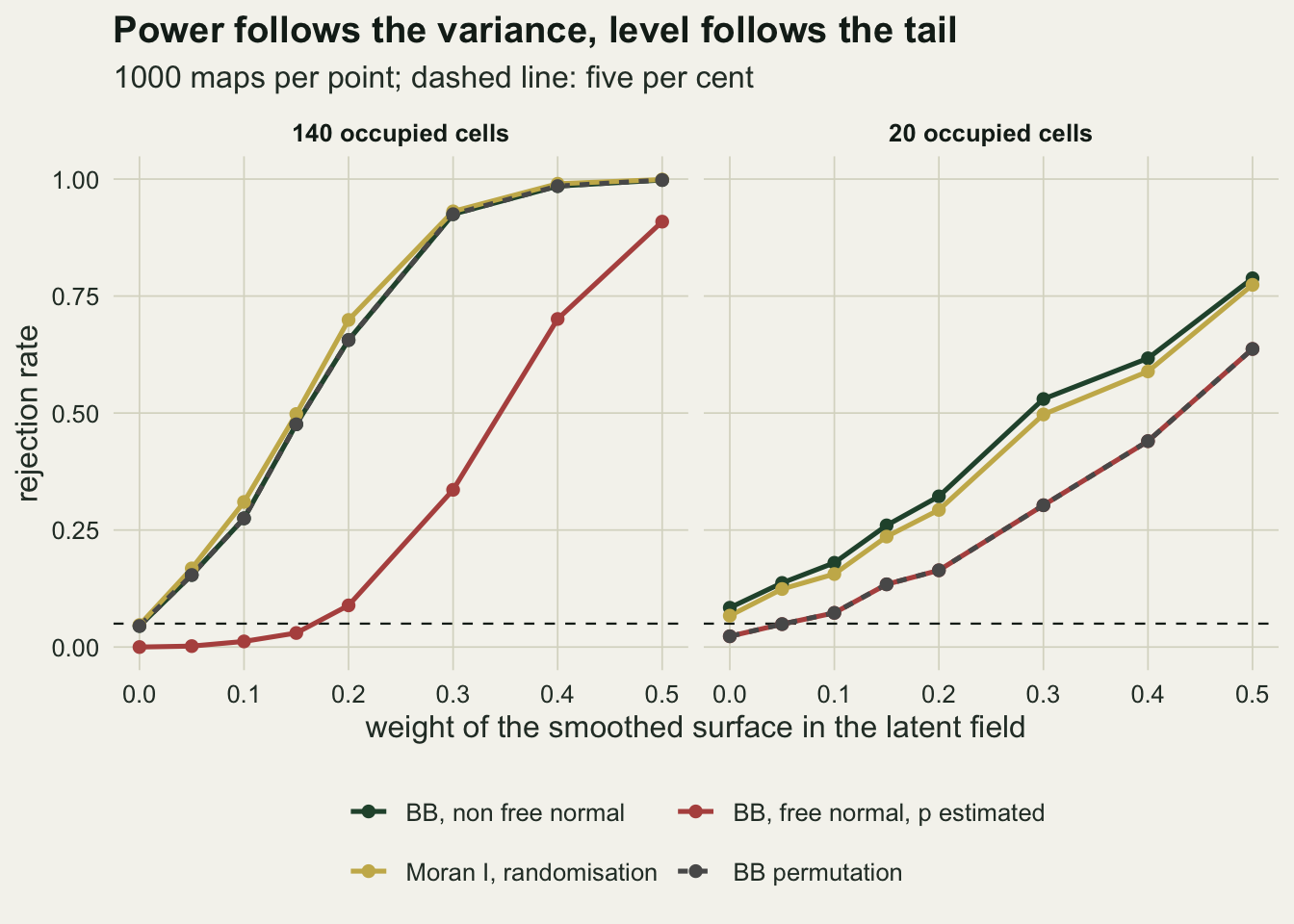
What to report
Report the three join counts, the number of occupied cells and the neighbour rule, because every expectation and variance depends on all of them. A rook grid and a queen grid give different join totals for the same map, and so do grids with and without a buffer of unsurveyed cells.
State which moments the z score uses. For a map whose number of occupied cells is known, the non free moments condition on that number and match the permutation distribution; the free sampling moments with an estimated prevalence gave a test that almost never rejected under the null and lost most of its power at moderate clustering on the 140 cell maps. If a paper or a package reports a join count z without saying which, the non free version is the one to ask for.
Moran’s I on the zero one vector is a defensible statistic on a grid like this one. It moved almost in lockstep with the BB count across permuted maps, and its randomisation z was close to the non free BB z on the example map. What it adds is familiarity to a reader; what the join counts add is an interpretation in joins that a field ecologist can check by eye on the map.
Use a permutation p value whenever the map is sparse. At a prevalence of five per cent on 400 cells the non free BB test and Moran’s I with either variance had levels between 0.068 and 0.101, and only the placing of the integers kept the free test in line with the permutation test. The permutation test needs no more code than the join count itself. Report the number of permutations and the resulting floor on the p value.
Honest limits
The grid is twenty by twenty with rook joins and no missing cells. Irregular survey units, queen neighbours and distance weights all change the join totals and the shared cell count, and the sizes of the normal approximation failure measured here depend on those totals. The sawtooth in the level sweep in particular is specific to this grid: another grid will have its teeth in other places.
The clustered maps come from one generator, a thresholded and smoothed Gaussian field. That produces blob shaped patches of occupied cells. Linear structures such as occupied cells along a hedgerow or a stream, or regular spacing from territorial exclusion, are different alternatives; the second one shows up as too many BW joins, and every test in this post was one sided in the clustering direction.
The generator is not quite stationary either. Averaging with fewer neighbours leaves edge and corner cells with more latent variance, and the rescaling is per map, not per cell, so the clustered alternative carries a slight preference for boundary cells as well as clustering.
The prevalence in the maps was set exactly by marking the highest latent cells. That is the non free sampling model by construction, so the power comparison favours the conditional tests in their own setting. The Bernoulli maps in the plug in section were the check under free sampling, and the non free test held its level there too, but only at a single prevalence of 0.35.
Imperfect detection is ignored. A stonechat survey misses territories, and missed presences thin out the BB joins in the same way that a lower prevalence does. The join count then tests the arrangement of detections, and a spatial pattern in detection probability, such as a survey route that runs along one side of the reserve, would show up as clustering of the species. Repeat visits and an occupancy likelihood separate detection from presence; the occupancy post linked above does that with a constant detection probability, and a spatial pattern in detection would need detection covariates as well.
Finally, a significant join count is evidence of spatial structure in the map, not of any process. A covariate with its own spatial pattern, such as soil moisture or distance to scrub, produces clustered presences with no interaction among territories at all. The test answers whether the pattern is random. Legendre 1993 made the case that spatial structure in ecological data is both a nuisance for classical tests and information about the processes behind it, and a join count only establishes that the structure is there; the modelling starts after it.
References
Moran PAP 1948 Journal of the Royal Statistical Society Series B 10(2):243-251 (10.1111/j.2517-6161.1948.tb00012.x)
Moran PAP 1950 Biometrika 37(1-2):17-23 (10.1093/biomet/37.1-2.17)
Cliff AD, Ord JK 1981 Spatial Processes: Models and Applications (ISBN 978-0-85086-081-8)
Legendre P 1993 Ecology 74(6):1659-1673 (10.2307/1939924)