library(ggplot2)
library(grid)

res_raw <- function(x, y) {
  1.5 * exp(-((x - 36)^2 + (y - 64)^2) / (2 * 22^2)) +
  1.2 * exp(-((x - 70)^2 + (y - 38)^2) / (2 * 24^2)) +
  (-0.00034) * ((x - 50)^2 + (y - 50)^2)
}
gx <- seq(0, 100, length.out = 120)
grid_df <- expand.grid(x = gx, y = gx)
grid_df$raw <- res_raw(grid_df$x, grid_df$y)
mu_r <- mean(grid_df$raw); sd_r <- sd(grid_df$raw)
resource <- function(x, y) (res_raw(x, y) - mu_r) / sd_r

rvm <- function(n, mu, kappa) {
  out <- numeric(n); a <- 1 + sqrt(1 + 4 * kappa^2)
  b <- (a - sqrt(2 * a)) / (2 * kappa); r <- (1 + b^2) / (2 * b)
  for (i in seq_len(n)) {
    repeat {
      u1 <- runif(1); u2 <- runif(1); u3 <- runif(1)
      z <- cos(pi * u1); f <- (1 + r * z) / (r + z); cc <- kappa * (r - f)
      if (cc * (2 - cc) - u2 > 0 || log(cc / u2) + 1 - cc >= 0) break
    }
    out[i] <- sign(u3 - 0.5) * acos(f) + mu
  }
  ((out + pi) %% (2 * pi)) - pi
}Integrated step selection analysis in R
movement ecology
habitat selection
R
ecology tutorial
Integrated step selection analysis from scratch: add movement covariates to a conditional model to debias habitat selection and recover the movement kernel.
The previous post left a loose end. A basic step selection function draws its available steps from a movement kernel fitted to the observed steps, but the observed steps are already the product of both movement and habitat selection. The fitted kernel is therefore contaminated, and the habitat coefficient inherits a small bias. Integrated step selection analysis, set out by Avgar and colleagues (2016) on foundations from Forester and colleagues (2009), closes the gap. The idea is disarmingly simple: put movement quantities into the model as covariates. Their coefficients pull the contaminated kernel back to the truth, and in doing so they lift the bias off the habitat coefficient.
A track with a known movement kernel
We simulate as before. The animal has a true movement kernel, a gamma for step length and a von Mises for turning angle, and it selects for a resource with a known strength. Every step is drawn from the movement kernel and then reweighted by the resource, which is the generative form of step selection.
k_true <- 2.0; th_true <- 6.0; lam_true <- 1 / th_true; kap_true <- 0.9
beta_true <- 1.0
n <- 1500; M <- 300
set.seed(5150)
pos <- matrix(NA_real_, n + 1, 2); pos[1, ] <- c(45, 52)
heading <- numeric(n + 1); heading[1] <- runif(1, -pi, pi)
for (i in 1:n) {
  L <- rgamma(M, shape = k_true, scale = th_true)
  a <- rvm(M, 0, kap_true)
  ang <- heading[i] + a
  ex <- pos[i, 1] + L * cos(ang); ey <- pos[i, 2] + L * sin(ang)
  w <- exp(beta_true * resource(ex, ey))
  j <- sample.int(M, 1, prob = w)
  pos[i + 1, ] <- c(ex[j], ey[j]); heading[i + 1] <- ang[j]
}
dx <- diff(pos[, 1]); dy <- diff(pos[, 2])
obs_l <- sqrt(dx^2 + dy^2)
bearing <- atan2(dy, dx)
obs_turn <- ((diff(bearing) + pi) %% (2 * pi)) - pi
The true movement kernel has shape 2, scale 6 and concentration 0.9. Now we do what a basic analysis does: fit a tentative kernel to the observed steps, matching moments for the gamma and the mean resultant length for the von Mises.
m1 <- mean(obs_l); v1 <- var(obs_l)
k0 <- m1^2 / v1; th0 <- v1 / m1; lam0 <- 1 / th0
C <- mean(cos(obs_turn)); S <- mean(sin(obs_turn)); Rbar <- sqrt(C^2 + S^2)
mu0 <- atan2(S, C)
kap0 <- if (Rbar < 0.53) 2 * Rbar + Rbar^3 + 5 * Rbar^5 / 6 else
        if (Rbar < 0.85) -0.4 + 1.39 * Rbar + 0.43 / (1 - Rbar) else
        1 / (Rbar^3 - 4 * Rbar^2 + 3 * Rbar)
The observed steps imply a gamma with shape 2.09 and scale 5.06, and a von Mises with concentration 0.73. Compare those to the truth: the scale has shrunk from 6 to 5.06 and the concentration from 0.9 to 0.73. Selection has bent the observed steps away from the movement kernel that produced them, which is exactly the contamination we need to remove.
The basic fit, and its bias
First the basic step selection function: one used step against K available steps drawn from the tentative kernel, habitat as the only covariate, conditional logistic likelihood. The likelihood machinery is the one built in the previous post.
K <- 12
set.seed(20260713)
use_idx <- 2:n
n_str <- length(use_idx)
p <- 4
X <- matrix(NA_real_, n_str * (K + 1), p)   # columns: resource, log_l, l, cos_turn
row <- 1
for (s in seq_along(use_idx)) {
  i <- use_idx[s]
  lu <- obs_l[i]; tu <- obs_turn[i - 1]
  zu <- resource(pos[i + 1, 1], pos[i + 1, 2])
  X[row, ] <- c(zu, log(lu), lu, cos(tu)); row <- row + 1
  Ls <- rgamma(K, shape = k0, scale = th0)
  As <- rvm(K, mu0, kap0)
  ang <- heading[i] + As
  ex <- pos[i, 1] + Ls * cos(ang); ey <- pos[i, 2] + Ls * sin(ang)
  X[row:(row + K - 1), ] <- cbind(resource(ex, ey), log(Ls), Ls, cos(As))
  row <- row + K
}

nll <- function(b, cols) {
  eta <- as.vector(X[, cols, drop = FALSE] %*% b)
  em <- matrix(eta, nrow = K + 1)          # column = stratum, row 1 = used step
  -sum(em[1, ] - log(colSums(exp(em))))
}
opt0 <- optim(0, nll, cols = 1, method = "BFGS", hessian = TRUE, control = list(reltol = 1e-10))
b_ssf <- opt0$par; se_ssf <- sqrt(1 / opt0$hessian[1, 1])
The basic estimate of habitat selection is 0.919, comfortably below the true value of 1. Nothing is wrong with the code; the bias comes entirely from the availability distribution being fitted to steps that selection has already shaped.
Adding movement to the model
Here is the whole of integrated step selection analysis. Write the density of a step as a movement kernel times a habitat term. A gamma movement kernel contributes (k - 1) log(l) - l / theta to the log density, and a von Mises kernel contributes kappa cos(a). When we sample available steps from a tentative kernel with shape k0, scale theta0 and concentration kappa0, the log ratio between the true redistribution kernel and the tentative sampling density is linear in the resource and in three movement quantities:
\[ \log \frac{\text{true}}{\text{tentative}} = \beta_z\, z + (k - k_0)\log l + (\lambda_0 - \lambda)\, l + (\kappa - \kappa_0)\cos a . \]
So we add log(l), l and cos(a) to the design alongside the resource, fit the same conditional logistic model, and read the true movement parameters straight off the coefficients:
\[ \hat k = k_0 + \beta_{\log l}, \qquad \hat\lambda = \lambda_0 - \beta_{l}, \qquad \hat\kappa = \kappa_0 + \beta_{\cos} . \]
opt1 <- optim(rep(0, p), nll, cols = 1:p, method = "BFGS", hessian = TRUE,
              control = list(reltol = 1e-10))
b <- opt1$par
se <- sqrt(diag(solve(opt1$hessian)))
names(b) <- c("resource", "log_l", "l", "cos_turn")

shape_hat <- k0 + b["log_l"]
rate_hat  <- lam0 - b["l"]
scale_hat <- 1 / rate_hat
kappa_hat <- kap0 + b["cos_turn"]
The habitat coefficient is now 1.001, sitting on the true value of 1; the bias is gone. The movement covariates have done their job. The corrected step-length kernel has shape 2.08 and scale 5.6, against a true scale of 6 and a contaminated tentative scale of 5.06, and the corrected concentration is 0.92 against a true 0.9 and a tentative 0.73. The model has recovered the animal’s underlying movement, not the movement plus selection that the raw steps show.
ll <- seq(0.1, max(obs_l) * 1.02, length.out = 300)
dens_l <- rbind(
  data.frame(kernel = "observed (tentative)", l = ll, d = dgamma(ll, shape = k0, scale = th0)),
  data.frame(kernel = "iSSA corrected", l = ll, d = dgamma(ll, shape = shape_hat, scale = scale_hat)),
  data.frame(kernel = "true", l = ll, d = dgamma(ll, shape = k_true, scale = th_true)))
dens_l$kernel <- factor(dens_l$kernel, levels = c("observed (tentative)", "iSSA corrected", "true"))
cols3 <- c("observed (tentative)" = "#b5534e", "iSSA corrected" = "#275139", "true" = "#16241d")
lty3  <- c("observed (tentative)" = "solid", "iSSA corrected" = "solid", "true" = "22")
pa <- ggplot(dens_l, aes(l, d, colour = kernel, linetype = kernel)) +
  geom_line(linewidth = 0.7) +
  scale_colour_manual(values = cols3) + scale_linetype_manual(values = lty3) +
  labs(x = "step length", y = "density", colour = NULL, linetype = NULL, title = "Step-length kernel") +
  theme_minimal(base_size = 11) +
  theme(panel.grid.minor = element_blank(), legend.position = c(0.66, 0.82),
        legend.background = element_rect(fill = "#ffffff", colour = NA),
        plot.title = element_text(size = 10, colour = "#46604a"))
aa <- seq(-pi, pi, length.out = 300)
vm <- function(a, kappa) exp(kappa * cos(a)) / (2 * pi * besselI(kappa, 0))
dens_a <- rbind(
  data.frame(kernel = "observed (tentative)", a = aa, d = vm(aa, kap0)),
  data.frame(kernel = "iSSA corrected", a = aa, d = vm(aa, kappa_hat)),
  data.frame(kernel = "true", a = aa, d = vm(aa, kap_true)))
dens_a$kernel <- factor(dens_a$kernel, levels = c("observed (tentative)", "iSSA corrected", "true"))
pb <- ggplot(dens_a, aes(a, d, colour = kernel, linetype = kernel)) +
  geom_line(linewidth = 0.7) +
  scale_colour_manual(values = cols3) + scale_linetype_manual(values = lty3) +
  scale_x_continuous(breaks = c(-pi, -pi/2, 0, pi/2, pi), labels = c("-pi", "-pi/2", "0", "pi/2", "pi")) +
  labs(x = "turning angle", y = "density", colour = NULL, linetype = NULL, title = "Turning-angle kernel") +
  theme_minimal(base_size = 11) +
  theme(panel.grid.minor = element_blank(), legend.position = "none",
        plot.title = element_text(size = 10, colour = "#46604a"))
grid.newpage(); pushViewport(viewport(layout = grid.layout(1, 2)))
print(pa, vp = viewport(layout.pos.row = 1, layout.pos.col = 1))
print(pb, vp = viewport(layout.pos.row = 1, layout.pos.col = 2))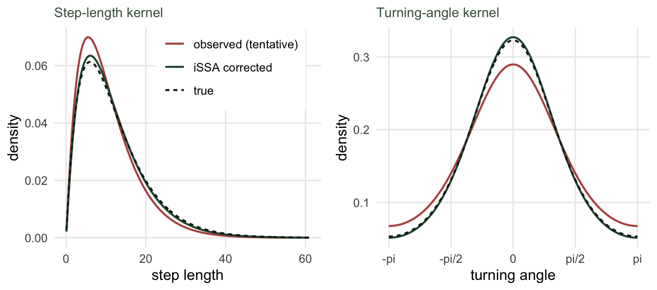
Effect size and what to report
Because habitat selection is now clean, its exponent is a relative selection strength worth quoting (Avgar and colleagues 2017). The basic fit gives 2.51 for a one standard deviation increase in the resource, while the integrated fit gives 2.72, close to the true value of 2.72. The gap between the two is the movement contamination expressed on the scale people actually report.
coef_df <- data.frame(
  model = factor(c("iSSA (movement + habitat)", "basic SSF (habitat only)"),
                 levels = c("basic SSF (habitat only)", "iSSA (movement + habitat)")),
  est = c(b["resource"], b_ssf), se = c(se["resource"], se_ssf))
ggplot(coef_df, aes(est, model)) +
  geom_vline(xintercept = beta_true, linetype = "dashed", colour = "#b5534e") +
  geom_errorbarh(aes(xmin = est - 1.96 * se, xmax = est + 1.96 * se),
                 height = 0.14, colour = "#275139", linewidth = 0.6) +
  geom_point(colour = "#275139", size = 2.8) +
  annotate("text", x = beta_true, y = 2.4, label = "true selection",
           colour = "#b5534e", size = 3, hjust = 1.05) +
  labs(x = "habitat selection coefficient", y = NULL) +
  theme_minimal(base_size = 11) + theme(panel.grid.minor = element_blank())
Warning: `geom_errorbarh()` was deprecated in ggplot2 4.0.0.
ℹ Please use the `orientation` argument of `geom_errorbar()` instead.`height` was translated to `width`.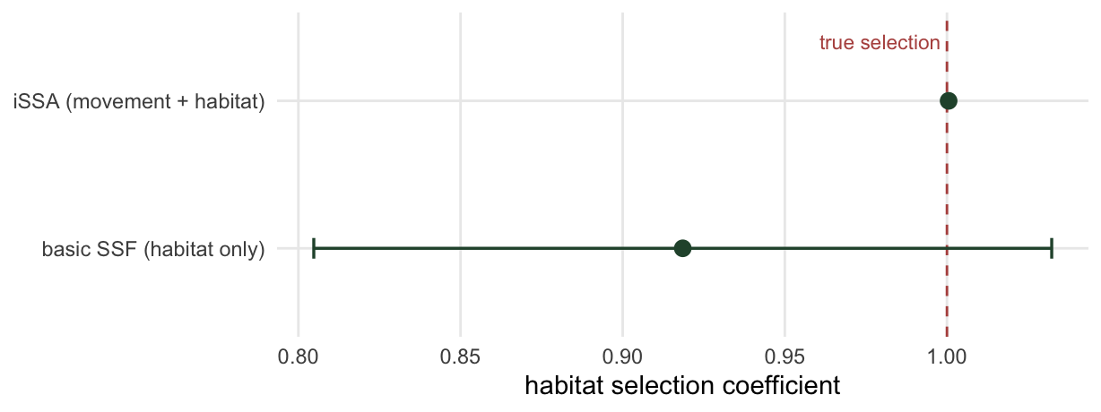
What this does and does not fix
The three movement covariates here assume a gamma step length and a symmetric von Mises turn. A directional bias, a tendency to keep turning one way, needs sin(a) as well; a step length whose spread changes with habitat needs interactions between the movement terms and the covariates. The tentative kernel still matters too: it should cover the range of steps the animal actually took, or the available set will miss part of the choice. That question, how many available steps and drawn from what, is the next post. What integrated step selection analysis buys, for the price of three extra columns, is a movement kernel and a habitat coefficient that no longer contaminate each other.
References
Avgar T, Potts JR, Lewis MA, Boyce MS 2016. Methods in Ecology and Evolution 7(5):619-630 (10.1111/2041-210X.12528).
Forester JD, Im HK, Rathouz PJ 2009. Ecology 90(12):3554-3565 (10.1890/08-0874.1).
Avgar T, Lele SR, Keim JL, Boyce MS 2017. Ecology and Evolution 7(14):5322-5330 (10.1002/ece3.3122).
Fieberg J, Signer J, Smith B, Avgar T 2021. Journal of Animal Ecology 90(5):1027-1043 (10.1111/1365-2656.13441).
Signer J, Fieberg J, Avgar T 2019. Ecology and Evolution 9(2):880-890 (10.1002/ece3.4823).
Fortin D, Beyer HL, Boyce MS, Smith DW, Duchesne T, Mao JS 2005. Ecology 86(5):1320-1330 (10.1890/04-0953).