library(ggplot2)

te_paper  <- "#f5f4ee"
te_ink    <- "#16241d"
te_body   <- "#2c3a31"
te_forest <- "#275139"
te_rust   <- "#b5534e"
te_gold   <- "#c9b458"
te_line   <- "#dad9ca"

theme_datasheet <- function() {
  theme_minimal(base_size = 12) +
    theme(plot.background  = element_rect(fill = te_paper, colour = NA),
          panel.background = element_rect(fill = te_paper, colour = NA),
          panel.grid.major = element_line(colour = te_line, linewidth = 0.3),
          panel.grid.minor = element_blank(),
          text             = element_text(colour = te_body),
          plot.title       = element_text(colour = te_ink, face = "bold"),
          plot.subtitle    = element_text(colour = te_body),
          axis.text        = element_text(colour = te_body),
          strip.text       = element_text(colour = te_ink))
}Integrated biomarker response and axis order
R
ecotoxicology
biomarkers
composite indices
simulation
ecology tutorial
The axis order of an IBR star plot can change the most impacted station, but a repeat survey changes it more often. Measured in R against a mean of z-scores.
Mussels are caged for six weeks at six stations along an estuary, from a clean inlet to the outfall below a harbour. Back in the laboratory each animal gives six biomarker values: an enzyme of phase II detoxification, an antioxidant enzyme, lipid peroxidation, metallothionein, a DNA damage score and an inhibited acetylcholinesterase whose sign is flipped so that larger means worse. The report needs one number per station and a sentence naming the most impacted one. A widely used number for that job is the Integrated Biomarker Response of Beliaeff and Burgeot (2002): standardise the station means of each biomarker, shift them so that the lowest station sits at zero, draw the six values as the spokes of a star plot, and add up the areas of the six triangles between neighbouring spokes.
An area depends on which spokes are neighbours. A station that scores high on two biomarkers gains a large triangle if those two spokes sit next to each other and two thin ones if they sit on opposite sides of the star. Sanchez et al. (2013) wrote that the IBR depends strongly on the arrangement of the biomarkers on the star and proposed the IBRv2, which measures each station’s deviation from a reference station and adds up the absolute deviations, so no order enters. Devin et al. (2014) reviewed how the IBR had been used and proposed a simpler formula together with a permutation procedure. Neither of those points is new here. What this post measures is how much the order matters next to the two other things that move the answer: the animals that happened to be caught, and the choice of index. The measured comparison is the post’s own content; the order dependence itself is the published result it demonstrates.
The site already has the pieces on either side. Ranking sites when every estimate is noisy shows how often the site ranked first by one noisy metric is the truly best one, with no composite involved. Structured decision making in R shows that the rule used to put objectives on a common scale can change which option wins, and Ecosystem multifunctionality and its threshold shows that the reference value used to standardise functions moves where the diversity effect peaks. None of the three has a geometry in it. The IBR adds one unreported choice, the axis order, and the question is what that choice costs in the currency of the other two.
Six biomarkers, six stations and sixty stars
The simulated stations lie on one contamination gradient, from 0 at the clean inlet to 2 at the outfall in equal steps. Each biomarker responds to the gradient with its own slope, drawn uniformly between 0.3 and 1 in units of the between-animal standard deviation, so every biomarker is informative and some are more so than others. On top of the gradient every station has its own departure on every biomarker, a normal deviation with standard deviation 0.25, 0.5 or 1: food, temperature, salinity and whatever else makes a station more than its position on the gradient. Individual animals then scatter around the station value with standard deviation 1, and 5, 10 or 20 animals are measured per station. The values are on the log scale in which biomarker data are usually analysed. The truly most impacted station is the outfall, station 6, by construction. The design constants were fixed before the simulations were run; the replication and the seeds were set once when the post was written and not changed.
With six axes there are 5! = 120 ways to arrange the spokes around the circle once rotations are ignored, and each arrangement read clockwise is the same star as its mirror image read anticlockwise, so (k - 1)!/2 = 60 stars differ in which spokes are neighbours. The code enumerates all of them by fixing biomarker 1 on the first spoke and keeping one of each mirror pair.
k_bm     <- 6
n_st     <- 6
grad     <- seq(0, 2, length.out = n_st)
slope_lo <- 0.3
slope_hi <- 1
resid_sd <- c(0.25, 0.5, 1)
n_animal <- c(5, 10, 20)
n_rep    <- 400

perm_rest <- as.matrix(expand.grid(rep(list(2:k_bm), k_bm - 1)))
perm_rest <- perm_rest[apply(perm_rest, 1, function(r) length(unique(r)) == k_bm - 1), ]
perm_rest <- perm_rest[perm_rest[, 1] < perm_rest[, k_bm - 1], ]
axis_orders <- cbind(1, perm_rest)
n_ord <- nrow(axis_orders)
next_spoke <- c(2:k_bm, 1)

ibr_scores <- function(site_means) {
  z_bm <- scale(site_means)
  s_bm <- sweep(z_bm, 2, apply(z_bm, 2, min))
  area <- apply(axis_orders, 1, function(o) {
    s_o <- s_bm[, o, drop = FALSE]
    rowSums(s_o * s_o[, next_spoke])
  })
  area * sin(2 * pi / k_bm) / 2
}
mean_z <- function(site_means) rowMeans(scale(site_means))
ibr_v2 <- function(site_means, animal_sd, ref_means) {
  rowSums(abs(sweep(sweep(site_means, 2, ref_means), 2, animal_sd, "/")))
}

draw_truth <- function(rsd, gradient = TRUE) {
  slopes <- runif(k_bm, slope_lo, slope_hi)
  g_used <- if (gradient) grad else rep(0, n_st)
  outer(g_used, slopes) + matrix(rnorm(n_st * k_bm, 0, rsd), n_st, k_bm)
}
draw_survey <- function(truth, n_an) {
  array(rnorm(n_st * k_bm * n_an, rep(truth, n_an), 1), c(n_st, k_bm, n_an))
}
ibr_scores() returns one IBR per station and per arrangement, a 6 by 60 matrix. The standardisation follows Beliaeff and Burgeot: the mean and standard deviation are taken over the station means of each biomarker, and the shift adds the absolute value of the lowest standardised score. The mean standardised score mean_z() uses the same standardised values and no geometry; because the shift is the same for every station, ranking by it is the same as ranking by the sum of the shifted spokes. For the IBRv2 the values are already on the log scale, so the log ratio to the reference station is a difference, and it is divided by the standard deviation of all individual values of that biomarker, stations lumped together; the reference is station 1, the clean inlet (the reference station itself is not a candidate).
One survey, two stars
Before any rates, one survey in which the order matters. The chunk below draws surveys with a station departure of 0.5 and 10 animals per station until it meets the first in which the top station is not the same under all 60 arrangements, then keeps that one.
set.seed(4417)
n_tried <- 0
repeat {
  n_tried <- n_tried + 1
  ex_truth  <- draw_truth(0.5)
  ex_survey <- draw_survey(ex_truth, 10)
  ex_means  <- apply(ex_survey, c(1, 2), mean)
  ex_ibr    <- ibr_scores(ex_means)
  ex_top    <- apply(ex_ibr, 2, which.max)
  if (length(unique(ex_top)) > 1) break
}
ex_tab   <- tabulate(ex_top, n_st)
ord_a    <- which(ex_top == which.max(ex_tab))[1]
ord_b    <- which(ex_top != which.max(ex_tab))[1]
ex_mz    <- mean_z(ex_means)
bm_share <- 100 * ex_tab / n_ord
The example took 8 draws. In it, station 6 has the largest IBR under 56 of the 60 arrangements and station 5 under the other 4. The mean standardised score ranks station 6 first. Figure 1 draws the six stations as stars under one arrangement of each kind.
star_df <- function(ord_idx, lab) {
  z_bm <- scale(ex_means)
  s_bm <- sweep(z_bm, 2, apply(z_bm, 2, min))
  o <- axis_orders[ord_idx, ]
  ang <- pi / 2 - 2 * pi * (seq_len(k_bm) - 1) / k_bm
  do.call(rbind, lapply(seq_len(n_st), function(st) {
    data.frame(station = paste("station", st), arrangement = lab,
               x = s_bm[st, o] * cos(ang), y = s_bm[st, o] * sin(ang),
               bm = paste0("B", o), spoke_x = max(s_bm) * 1.18 * cos(ang),
               spoke_y = max(s_bm) * 1.18 * sin(ang),
               top = st == ex_top[ord_idx],
               ibr = ex_ibr[st, ord_idx])
  }))
}
lab_a <- paste("order", paste0("B", axis_orders[ord_a, ], collapse = " "))
lab_b <- paste("order", paste0("B", axis_orders[ord_b, ], collapse = " "))
stars <- rbind(star_df(ord_a, lab_a), star_df(ord_b, lab_b))
stars$arrangement <- factor(stars$arrangement, levels = c(lab_a, lab_b))
star_lab <- unique(stars[, c("station", "arrangement", "ibr", "top")])
ggplot(stars, aes(x, y)) +
  geom_segment(aes(x = 0, y = 0, xend = spoke_x, yend = spoke_y),
               colour = te_line, linewidth = 0.3) +
  geom_text(aes(spoke_x * 1.12, spoke_y * 1.12, label = bm), size = 2.3,
            colour = te_body) +
  geom_polygon(aes(fill = top), colour = te_ink, linewidth = 0.4, alpha = 0.85) +
  geom_text(data = star_lab, aes(x = 0, y = -max(stars$spoke_y) * 1.55,
                                 label = sprintf("%.2f", ibr)),
            size = 3, colour = te_ink) +
  facet_grid(arrangement ~ station) +
  scale_fill_manual(values = c("FALSE" = te_line, "TRUE" = te_rust), guide = "none") +
  coord_equal(clip = "off") +
  labs(x = NULL, y = NULL, title = "Same survey, two arrangements of the spokes") +
  theme_datasheet() +
  theme(axis.text = element_blank(), panel.grid.major = element_blank(),
        strip.text.y = element_text(size = 8))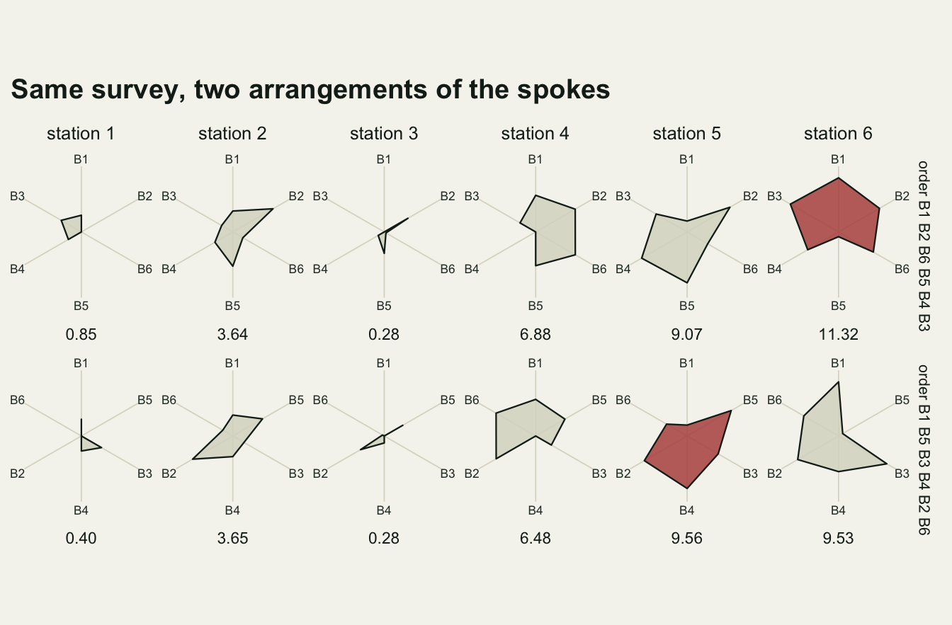
That is the published result, and one example is enough to establish it. It says nothing about how often it happens or whether it matters, which needs many surveys.
Order noise against survey noise
For each of the nine cells, 400 surveys are simulated. In each survey the IBR is computed under all 60 arrangements, and a second, independent survey of new animals from the same stations is drawn. Two denominators are needed and both are kept. Per survey: is the top station the same under every arrangement, and what share of the 60 arrangements disagrees with the most common top station? Per pair: if two analysts pick two different arrangements at random for the same data, how often do they name different top stations; and if one analyst keeps the arrangement and surveys again, how often does the top station change? The two pairwise rates are directly comparable, because each is the probability that one change, of arrangement or of animals, moves the answer.
one_survey <- function(rsd, n_an, gradient = TRUE) {
  truth <- draw_truth(rsd, gradient)
  surv1 <- draw_survey(truth, n_an)
  surv2 <- draw_survey(truth, n_an)
  m1 <- apply(surv1, c(1, 2), mean)
  m2 <- apply(surv2, c(1, 2), mean)
  ibr1 <- ibr_scores(m1)
  top1 <- apply(ibr1, 2, which.max)
  top2 <- apply(ibr_scores(m2), 2, which.max)
  p_top <- tabulate(top1, n_st) / n_ord
  sd_pool <- apply(surv1, 2, sd)
  v2_est  <- ibr_v2(m1, sd_pool, m1[1, ])
  v2_true <- ibr_v2(m1, sd_pool, truth[1, ])
  c(any_dep      = length(unique(top1)) > 1,
    arr_disagree = 1 - max(p_top),
    order_swap   = (1 - sum(p_top^2)) * n_ord / (n_ord - 1),
    survey_swap  = mean(top1 != top2),
    mz_survey    = which.max(mean_z(m1)) != which.max(mean_z(m2)),
    ibr_worst    = mean(top1 == n_st),
    mz_worst     = which.max(mean_z(m1)) == n_st,
    perm_worst   = which.max(rowMeans(ibr1)) == n_st,
    v2_worst     = which.max(v2_est[-1]) + 1 == n_st,
    v2t_worst    = which.max(v2_true[-1]) + 1 == n_st,
    v2s_worst    = which.max(rowSums(sweep(sweep(m1, 2, m1[1, ]), 2, sd_pool, "/"))[-1]) + 1 == n_st)
}

cells <- expand.grid(rsd = resid_sd, n_an = n_animal)
set.seed(2002)
runs <- lapply(seq_len(nrow(cells)), function(i)
  replicate(n_rep, one_survey(cells$rsd[i], cells$n_an[i])))
res <- cbind(cells, t(sapply(runs, rowMeans)))
mc_se <- function(p) sqrt(p * (1 - p) / n_rep)
cell_val <- function(col, rsd, n_an) res[res$rsd == rsd & res$n_an == n_an, col]
ratio_swap <- res$survey_swap / res$order_swap
order_hi_n <- range(res$order_swap[res$rsd == 1])
cond_dis   <- res$arr_disagree / res$any_dep
gap_se     <- sapply(runs, function(r) sd(r["survey_swap", ] - r["order_swap", ]) / sqrt(n_rep))
gap_in_se  <- (res$survey_swap - res$order_swap) / gap_se
Across the nine cells the top station depends on the arrangement in between 4 and 33 per cent of surveys. Counted per arrangement the effect is much smaller: the share of the 60 arrangements that disagree with the most common top station averages between 0.9 and 8.7 per cent. In a survey where the order matters, between 21 and 26 per cent of the arrangements name a different station, so the small per-arrangement average comes from the surveys the order leaves alone, not from a few stray arrangements in the surveys it affects.
The pairwise rates put this next to sampling. Two arrangements chosen at random disagree on the top station with probability 0.013 to 0.117; a repeat survey with the arrangement held fixed changes it with probability 0.148 to 0.331. In every cell the repeat survey moves the answer more often, by a factor of 1.6 in the cell where the two are closest and 13.9 where they are furthest apart. Both rates come from the same 400 surveys per cell, so the gap has a paired Monte Carlo standard error, at most 0.0216; the smallest gap is 5.1 paired standard errors wide. Dropping the geometry does not calm the animals either: the mean standardised score changes its top station under a repeat survey with probability 0.142 to 0.325.
The two kinds of noise answer to different parts of the design. More animals shrink the survey noise: at a station departure of 0.25 the repeat-survey rate falls from 0.331 with 5 animals to 0.176 with 20. Order noise is driven mainly by the station departures: with 20 animals it grows from 0.013 at a departure of 0.25 to 0.098 at 1, and at a departure of 1 it stays between 0.098 and 0.117 whatever the number of animals. More animals lower it at departures of 0.25 and 0.5 (from 0.039 to 0.013 at 0.25 and from 0.069 to 0.040 at 0.5) but not at 1. The more the biomarkers of a station disagree with each other, the more it matters which of them are neighbours. Figure 2 shows both.
swap_long <- rbind(
  data.frame(res[, c("rsd", "n_an")], rate = res$order_swap, kind = "another arrangement"),
  data.frame(res[, c("rsd", "n_an")], rate = res$survey_swap, kind = "another survey"))
swap_long$n_lab <- factor(paste(swap_long$n_an, "animals per station"),
                          levels = paste(n_animal, "animals per station"))
swap_long$se <- mc_se(swap_long$rate)
ggplot(swap_long, aes(factor(rsd), rate, colour = kind, group = kind)) +
  geom_line(linewidth = 0.8) +
  geom_errorbar(aes(ymin = rate - 2 * se, ymax = rate + 2 * se), width = 0.12,
                linewidth = 0.5) +
  geom_point(size = 2.4) +
  facet_wrap(~ n_lab, ncol = 3) +
  scale_colour_manual(values = c("another arrangement" = te_gold,
                                 "another survey" = te_forest), name = NULL) +
  scale_y_continuous(limits = c(0, NA)) +
  labs(x = "station departure from the gradient (sd)",
       y = "P(top station changes)",
       title = "The animals move the answer more than the spokes") +
  theme_datasheet() +
  theme(legend.position = "bottom")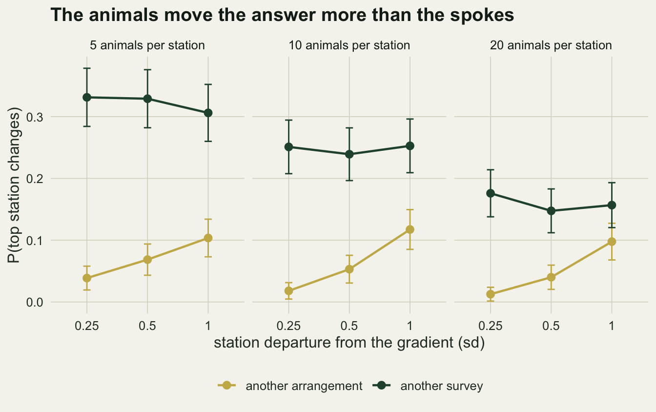
Which index finds the outfall
Stability is not the same as being right. The more useful question is how often each index names station 6, the station with the most contamination. For the IBR the answer is averaged over the 60 arrangements, which is what a reader facing an unreported arrangement should expect. The IBRv2 is scored in two versions: with the reference taken from the survey of station 1, as it would be in practice, and with the reference set to the true station 1 values, which removes the sampling noise of the reference animals (the reference station keeps its own departure). A third version drops the absolute value and adds the signed standardised deviations, to see what the absolute value costs.
diff_se <- sapply(runs, function(r) sd(r["ibr_worst", ] - r["mz_worst", ]) / sqrt(n_rep))
ibr_mz_gap <- res$ibr_worst - res$mz_worst
v2_gap_hi  <- res$mz_worst[res$rsd == 1] - res$v2_worst[res$rsd == 1]
v2_ref_gain <- (res$v2t_worst - res$v2_worst)[res$rsd == 1]
v2s_hi     <- res$v2s_worst[res$rsd == 1]
v2_hi      <- res$v2_worst[res$rsd == 1]
v2_gap_lo  <- res$mz_worst[res$rsd == 0.25] - res$v2_worst[res$rsd == 0.25]
perm_gap   <- res$perm_worst - res$mz_worst
The IBR names the outfall in 51 to 89 per cent of surveys and the mean standardised score in 52 to 90 per cent. Cell by cell the difference, IBR minus mean score, lies between -0.010 and 0.000, and the largest of the paired Monte Carlo standard errors of that difference is 0.008. The star plot adds no accuracy over an average of the numbers on its spokes. Averaging the IBR itself over the 60 arrangements, in the spirit of the permutation procedure of Devin et al., gives an order-free index whose hit rate differs from the mean score’s by between -0.003 and 0.008.
The IBRv2 with a surveyed reference is within 0.017 of the mean score when stations depart from the gradient by 0.25 and falls behind when they depart a lot: at a departure of 1 it names the outfall 0.102 to 0.145 less often than the mean score. At that departure, knowing the true reference values changes its hit rate by between -0.003 and 0.018, so most of that loss is not the few animals at the reference. The absolute value accounts for it: the IBRv2 counts a station that is lower than the reference on a biomarker as deviating just as much as one that is higher, and with large station departures the upstream stations collect deviations in both directions. With the signs kept, the same surveyed reference names the outfall in 0.522 to 0.570 of surveys at a departure of 1, against 0.372 to 0.415 for the IBRv2 itself.
worst_long <- rbind(
  data.frame(res[, c("rsd", "n_an")], hit = res$ibr_worst, index = "IBR, 60 arrangements"),
  data.frame(res[, c("rsd", "n_an")], hit = res$mz_worst, index = "mean standardised score"),
  data.frame(res[, c("rsd", "n_an")], hit = res$v2_worst, index = "IBRv2, surveyed reference"),
  data.frame(res[, c("rsd", "n_an")], hit = res$v2t_worst, index = "IBRv2, true reference"))
worst_long$index <- factor(worst_long$index, levels = unique(worst_long$index))
worst_long$n_lab <- factor(paste(worst_long$n_an, "animals per station"),
                           levels = paste(n_animal, "animals per station"))
ggplot(worst_long, aes(factor(rsd), hit, colour = index, group = index,
                       linetype = index)) +
  geom_line(linewidth = 0.8) +
  geom_point(size = 2.2) +
  facet_wrap(~ n_lab, ncol = 3) +
  scale_colour_manual(values = c(te_rust, te_forest, te_gold, te_gold), name = NULL) +
  scale_linetype_manual(values = c("solid", "22", "solid", "dotted"), name = NULL) +
  scale_y_continuous(limits = c(0.3, 1)) +
  labs(x = "station departure from the gradient (sd)",
       y = "P(names the outfall)",
       title = "The geometry adds nothing to the average") +
  guides(colour = guide_legend(nrow = 2), linetype = guide_legend(nrow = 2)) +
  theme_datasheet() +
  theme(legend.position = "bottom")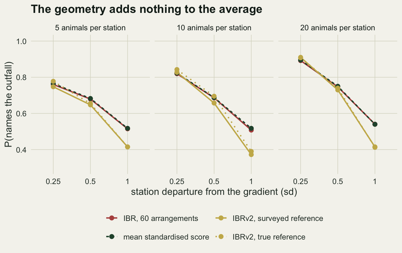
Without a gradient the order decides
The rates above are low because the stations share a gradient: when every biomarker points the same way, the station that is high on one is usually high on the rest and its star is large in every arrangement. Take the gradient away, so that the stations differ only by their departures, and the picture changes.
set.seed(1316)
flat <- rowMeans(replicate(n_rep, one_survey(1, 10, gradient = FALSE)))
With a station departure of 1, 10 animals per station and no gradient, the top station depends on the arrangement in 52 per cent of surveys, 15.6 per cent of arrangements disagree with the most common top station, and two random arrangements disagree with probability 0.210 against 0.321 for a repeat survey. The order still moves the answer less often than the animals do, but it is now a large share of the instability. There is no most impacted station to find in this arm, which is exactly the situation in which the arrangement has the most room: an index that is asked to rank stations that do not differ in a consistent direction will rank them by whatever it can.
A biomarker that turns back
A mean of standardised scores assumes that every biomarker, after its sign is set, rises with the stress. Some do not. An enzyme such as EROD can be induced at moderate exposure and inhibited at high exposure, so the most contaminated station scores low on it. The IBR assumes the same thing, since its spokes are the same standardised scores. The chunk below replaces biomarker 1 with such a response, rising to twice its slope in the middle of the gradient and falling back to zero at the outfall, and compares the hit rates with the monotone design and with the turning biomarker dropped. The cell is a station departure of 0.5 with 10 animals.
one_bell <- function(turning) {
  slopes <- runif(k_bm, slope_lo, slope_hi)
  resp <- outer(grad, slopes)
  if (turning) resp[, 1] <- 2 * slopes[1] * grad * (2 - grad)
  truth <- resp + matrix(rnorm(n_st * k_bm, 0, 0.5), n_st, k_bm)
  m1 <- apply(draw_survey(truth, 10), c(1, 2), mean)
  top1 <- apply(ibr_scores(m1), 2, which.max)
  c(ibr = mean(top1 == n_st), mz = which.max(mean_z(m1)) == n_st,
    mz_drop = which.max(mean_z(m1[, -1])) == n_st,
    dep = length(unique(top1)) > 1)
}
set.seed(2448)
bell_mono <- rowMeans(replicate(2 * n_rep, one_bell(FALSE)))
bell_turn <- rowMeans(replicate(2 * n_rep, one_bell(TRUE)))
bell_drop <- bell_mono - bell_turn
With every biomarker monotone the IBR names the outfall in 0.722 of 800 surveys and the mean score in 0.729. With biomarker 1 turning back those fall to 0.466 and 0.491, and the share of surveys whose top station depends on the arrangement goes from 0.156 to 0.324. Dropping the turning biomarker from the mean score brings the hit rate back to 0.699. The turning biomarker costs the IBR 0.256 and the mean score 0.237, similar amounts; the star plot has no way to recognise that one of its spokes is pointing the wrong way at the high end, and neither has the average. The shape of each response has to be known, from exposure experiments like those in Hormesis and non-monotonic responses, before either index is computed.
What to report
The IBR is a sum of products of neighbouring spokes, so its arrangement is part of the index. Give it: list the biomarkers in the order they were placed on the star, say why (by level of biological organisation, by the order in the protocol, or arbitrarily), and state whether the ranking of stations changes under the other arrangements. With six biomarkers there are only 60 arrangements, and computing all of them is a loop of a few lines, as ibr_scores() shows.
The larger instability comes from the animals, so the ranking needs an interval before it needs an arrangement. A bootstrap that resamples animals within each station and recomputes the index gives one. The chunk below does this for the example survey of Figure 1, with the arrangement of the upper row of stars held fixed, and records how often each station comes out on top; the same is tabulated over the 60 arrangements with the animals held fixed.
set.seed(1322)
n_boot <- 1000
n_ex_an <- dim(ex_survey)[3]
boot_top <- t(replicate(n_boot, {
  pick_an <- matrix(sample.int(n_ex_an, n_st * n_ex_an, replace = TRUE), n_st)
  bm_boot <- t(sapply(seq_len(n_st), function(st)
    rowMeans(ex_survey[st, , pick_an[st, ]])))
  ibr_b <- ibr_scores(bm_boot)
  c(ibr = which.max(ibr_b[, ord_a]), mz = which.max(mean_z(bm_boot)))
}))
boot_share_ibr <- tabulate(boot_top[, "ibr"], n_st) / n_boot
boot_share_mz  <- tabulate(boot_top[, "mz"], n_st) / n_boot
In the example, station 6 tops the IBR in 0.772 of the bootstrap resamples and station 5 in 0.207; the mean score puts them first in 0.681 and 0.307. Over the 60 arrangements with the animals fixed the split was 0.933 and 0.067. Figure 3 puts the three distributions side by side. A sentence naming one station as the most impacted is only supported when the bootstrap share for that station is large; the arrangement table is a check on a smaller source of doubt.
boot_df <- data.frame(
  station = factor(rep(seq_len(n_st), 3)),
  share = c(ex_tab / n_ord, boot_share_ibr, boot_share_mz),
  source = factor(rep(c("60 arrangements, same animals",
                        "bootstrap animals, IBR",
                        "bootstrap animals, mean score"), each = n_st),
                  levels = c("60 arrangements, same animals",
                             "bootstrap animals, IBR",
                             "bootstrap animals, mean score")))
ggplot(boot_df, aes(station, share, fill = source)) +
  geom_col(position = position_dodge(width = 0.8), width = 0.75) +
  scale_fill_manual(values = c(te_gold, te_forest, te_rust), name = NULL) +
  scale_y_continuous(limits = c(0, 1)) +
  labs(x = "station (6 = outfall)", y = "share naming the station first",
       title = "Which station is on top, and how sure") +
  guides(fill = guide_legend(nrow = 1)) +
  theme_datasheet() +
  theme(legend.position = "bottom")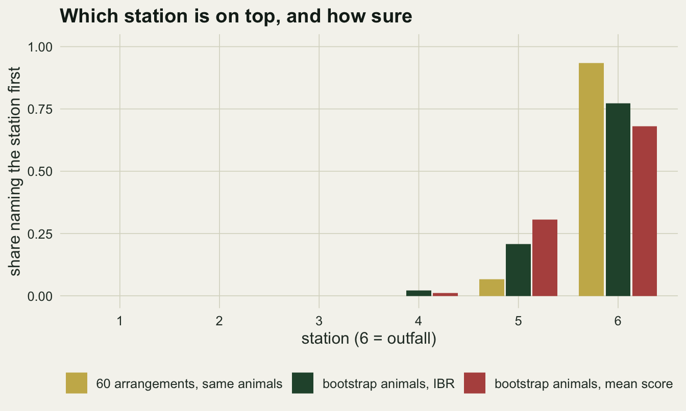
If the IBR is kept for its star plot, which is a readable picture of which biomarkers drive a station, report the mean standardised score beside it: in these simulations it found the most contaminated station as often as the IBR did, it needs no arrangement, and its bootstrap interval is easier to explain. Report the IBRv2 only with the reference named and its number of animals given, and do not read a large IBRv2 as more impact when stations can deviate from the reference in both directions.
Honest limits
The biomarkers are independent within an animal and the station departures are independent across biomarkers. Real biomarkers covary: two antioxidant enzymes answer the same oxidative stress, and correlated biomarkers placed next to each other give a station with that stress two large spokes side by side. Correlation changes both which spokes carry a station’s signal together and how noisy the station means are, and its effect on the order rates was not measured here; it can push them either way.
There is one gradient. Real estuaries have several stressors that load on different biomarkers, metals on metallothionein and organics on phase I and II enzymes, and a site with a different mixture is closer to the no-gradient arm than to the main design. The two arms bracket the question rather than answer it for a real survey.
Six biomarkers and six stations were fixed. The number of arrangements grows as (k - 1)!/2, 2520 for eight biomarkers, and with more spokes each triangle is a smaller part of the total, so the size of the order effect at other k is not measured here.
The truth is “the station with the most contamination”, and every index was scored against it. A regulator may want the station whose biological state is worst, which is the same station only when all biomarker responses are monotone and equally relevant; the turning-biomarker section shows one way they can differ, and there are others, such as an adapted population whose biomarkers are no longer induced.
The IBRv2 here uses the standard deviation of all individual log values, stations lumped together, and a single reference station. Published applications differ in how the reference is built (one site, several sites, a laboratory control) and in whether the standard deviation is taken over individuals or over site means, and both choices change its weights. Sanchez et al. (2013) compute the mean and standard deviation of the log ratios “as previously described by Beliaeff and Burgeot”, which leaves open whether they are taken over animals or over station means; the version here takes them over animals, and is one reading of the method rather than every variant in use.
Axis order is not always arbitrary in practice. Some studies place biomarkers by level of biological organisation or by function, which fixes one arrangement before the data are seen. That removes the choice from the analyst but not from the index: a different, equally sensible grouping is another of the 60 stars.
References
Beliaeff B, Burgeot T 2002 Environmental Toxicology and Chemistry 21(6):1316-1322 (10.1002/etc.5620210629)
Sanchez W, Burgeot T, Porcher JM 2013 Environmental Science and Pollution Research 20(5):2721-2725 (10.1007/s11356-012-1359-1)
Devin S, Burgeot T, Giamberini L, Minguez L, Pain-Devin S 2014 Environmental Science and Pollution Research 21(4):2448-2454 (10.1007/s11356-013-2169-9)