Choosing a factor smooth for a half-sampled group

When one group is sampled on half the gradient, the sz factor smooth runs an unpenalised line into the gap. Measuring in R which hierarchical GAMs hold up.

The six amphipod lakes of Hierarchical GAMs and factor smooths in mgcv come back with one change. The remote upland tarn still sends only eight animals, but this season the only incubators free at the field station run cold, and all eight are reared between 6 and 18 degrees. The five easy lakes are reared across the whole range, 6 to 30 degrees, as before. Every lake’s growth peaks somewhere near 21 degrees, so the tarn’s data stop below its optimum, and the question is what a hierarchical GAM says about the tarn’s warm half, where it has no animals at all.

That post names this case in its honest limits and leaves it open: “A tarn whose eight animals all came from the cold half of the range would test a different thing, the ability of the global curve to extrapolate a lake’s deviation, and the numbers above do not describe it.” Its last paragraph names a construction it did not fit, the "sz" factor smooth, whose group level smooths are constrained so that their equivalent coefficients sum to zero across groups, and calls it “the natural next comparison”. This post runs both at once: the half-sampled tarn, and "sz" next to the constructions the first post compared.

The pieces are not new. Checking a generalised additive model shows, for a single smooth, that outside the data mgcv follows the boundary behaviour of the basis, which for thin-plate and cubic regression splines is roughly a straight line; that the unpenalised part of a spline (its null space) carries that line is textbook material (Wood 2017). The hierarchical GAM post found that “a by smooth with m = 2 always keeps an unpenalised straight line per lake”, and that GI, with m = 1 on its group smooths, had the lowest error for the well sampled lakes. Pedersen et al (2019) use m = 1 for the group level smooths of their model GI for a different reason, to reduce collinearity with the global smooth, and do not discuss groups sampled over part of the range. The mgcv help presents "sz" as the construction that forces the main effect to do as much of the work as possible, and says nothing about a group whose data stop halfway. What this post measures is how those unpenalised pieces behave when the thing being extrapolated is a group’s deviation from a well supported global curve, for "sz" as the help writes it, and which constructions keep the tarn’s curve close to the global one where the tarn has no data.

library(mgcv)
library(ggplot2)
library(patchwork)

te_paper  <- "#f5f4ee"
te_ink    <- "#16241d"
te_body   <- "#2c3a31"
te_forest <- "#275139"
te_rust   <- "#b5534e"
te_gold   <- "#c9b458"
te_line   <- "#dad9ca"

theme_datasheet <- function() {
  theme_minimal(base_size = 12) +
    theme(plot.background  = element_rect(fill = te_paper, colour = NA),
          panel.background = element_rect(fill = te_paper, colour = NA),
          panel.grid.major = element_line(colour = te_line, linewidth = 0.3),
          panel.grid.minor = element_blank(),
          text             = element_text(colour = te_body),
          plot.title       = element_text(colour = te_ink, face = "bold"),
          plot.subtitle    = element_text(colour = te_body),
          axis.text        = element_text(colour = te_body),
          strip.text       = element_text(colour = te_ink, face = "bold"))
}

The tarn’s animals stop at 18 degrees

The generator is the one from the hierarchical GAM post, constant for constant: six lakes sharing an asymmetric curve whose fall above the optimum is twice as steep as its rise, lake optima drawn around 21 degrees, lake offsets, measurement noise, twelve animals in each of five lakes and eight in the tarn. The only change is that the tarn’s temperatures are drawn between two limits given as arguments; with the defaults the generator is the original one. The design constants were fixed before anything was fitted.

n_grp    <- 6                       # lake populations
n_full   <- 12                      # animals in each of the first five lakes
n_sparse <- 8                       # animals from the remote tarn
k_basis  <- 6                       # basis dimension for every smooth
t_lo <- 6; t_hi <- 30               # rearing range, degrees C
opt_mu <- 21; opt_sd <- 1.5         # lake optima
lev_sd <- 0.15                      # lake offsets
sd_eps <- 0.15                      # measurement noise
w_cool <- 6; w_warm <- 3            # curve width below and above the optimum
pop_lev    <- LETTERS[seq_len(n_grp)]
sparse_pop <- pop_lev[n_grp]
t_mid <- 18                         # the tarn's cold half ends here

tpc_true <- function(temp, opt, lev) {
  lev + exp(-0.5 * ((temp - opt) / ifelse(temp < opt, w_cool, w_warm))^2)
}

sim_pops <- function(tarn_lo = t_lo, tarn_hi = t_hi) {
  n_vec  <- c(rep(n_full, n_grp - 1), n_sparse)
  opt    <- rnorm(n_grp, opt_mu, opt_sd)
  lev    <- rnorm(n_grp, 0, lev_sd)
  pop    <- factor(rep(pop_lev, n_vec), levels = pop_lev)
  temp   <- runif(sum(n_vec), t_lo, t_hi)
  tarn   <- pop == sparse_pop
  temp[tarn] <- runif(sum(tarn), tarn_lo, tarn_hi)   # the one change
  gi     <- as.integer(pop)
  growth <- tpc_true(temp, opt[gi], lev[gi]) + rnorm(length(temp), 0, sd_eps)
  list(dat = data.frame(pop, temp, growth), opt = opt, lev = lev)
}

The models keep the names of Pedersen et al (2019) and of the first post. G is the global smooth with a random intercept per lake and no lake shape at all. GS adds a factor smooth ("fs", m = 2), whose penalties cover each lake’s constant and straight line as well as its wiggliness. GI adds by smooths with m = 1 and their own smoothing parameters, and GI_m2 is the same with m = 2. SZ is the "sz" factor smooth written as the mgcv help writes it: a smooth per lake with the default m = 2, a smoothing parameter per lake, and no separate lake term, because the help warns that “adding main effects or interactions of the factors will lead to a rank deficient model”. The "sz" smooths are not centred, so each lake’s constant lives inside its smooth. Four variants take SZ apart: SZ_id shares one smoothing parameter across the lakes, SZ_m1 lowers the penalty order to one, SZ_sel refits SZ with select = TRUE, which adds a penalty on the null space of every smooth in the model (Marra and Wood 2011), and SZ_ts penalises the null space of the "sz" term alone, by building its smooths on the shrinkage basis (xt = list(bs = "ts")). SZ_first is SZ with the tarn moved from the last factor level to the first. The sum to zero contrast writes the last level’s coefficients as minus the sum of the others, but mgcv gives every level, the last one included, its own penalty, so the model does not depend on the order; the relabelled fit only gives the optimiser a second start, and the worked example below shows why that matters. The last model, G_line, has no smooth at the lake level: the global smooth with a fixed intercept and an unpenalised least squares slope for each lake (the slopes sum to zero), which isolates the straight line. Every model is fitted by restricted maximum likelihood, the smoothing parameter estimation of Wood (2011).

form_list <- list(
  G     = growth ~ s(temp, k = k_basis, m = 2) + s(pop, bs = "re"),
  GS    = growth ~ s(temp, k = k_basis, m = 2) +
                   s(temp, pop, bs = "fs", k = k_basis, m = 2),
  GI    = growth ~ s(temp, k = k_basis, m = 2) +
                   s(temp, by = pop, k = k_basis, m = 1) + s(pop, bs = "re"),
  GI_m2 = growth ~ s(temp, k = k_basis, m = 2) +
                   s(temp, by = pop, k = k_basis, m = 2) + s(pop, bs = "re"),
  SZ    = growth ~ s(temp, k = k_basis, m = 2) + s(pop, temp, bs = "sz", k = k_basis),
  SZ_m1 = growth ~ s(temp, k = k_basis, m = 2) + s(pop, temp, bs = "sz", k = k_basis, m = 1),
  SZ_id = growth ~ s(temp, k = k_basis, m = 2) + s(pop, temp, bs = "sz", k = k_basis, id = 1)
)
form_list$SZ_sel   <- form_list$SZ           # fitted with select = TRUE
form_list$SZ_first <- form_list$SZ           # fitted with the tarn as the first level
form_list$SZ_ts    <- growth ~ s(temp, k = k_basis, m = 2) +
                      s(pop, temp, bs = "sz", k = k_basis, xt = list(bs = "ts"))
form_list$G_line   <- growth ~ s(temp, k = k_basis, m = 2) + pop + lin

# gam.side() reports nested smooths of the same variable; that message is expected here
quiet_gam <- function(form, dat, select = FALSE, ...) {
  withCallingHandlers(gam(form, data = dat, method = "REML", select = select, ...),
    warning = function(w) {
      if (grepl("repeated 1-d smooths", conditionMessage(w))) invokeRestart("muffleWarning")
    })
}

grid_t  <- seq(t_lo, t_hi, by = 0.25)
new_pop <- expand.grid(temp = grid_t, pop = factor(pop_lev, levels = pop_lev))
tarn_i  <- new_pop$pop == sparse_pop
first_lev <- c(sparse_pop, pop_lev[-n_grp])

# sum to zero slope columns: one unpenalised straight line per lake
lin_cols <- function(pop, temp) {
  X <- model.matrix(~ pop, contrasts.arg = list(pop = "contr.sum"))[, -1, drop = FALSE]
  X * temp
}
fit_model <- function(nm, dat) {
  nd <- new_pop
  if (nm == "SZ_first") {
    dat$pop <- factor(as.character(dat$pop), levels = first_lev)
    nd$pop  <- factor(as.character(nd$pop), levels = first_lev)
  }
  if (nm == "G_line") {
    dat$lin <- lin_cols(dat$pop, dat$temp)
    nd$lin  <- lin_cols(nd$pop, nd$temp)
  }
  fit <- quiet_gam(form_list[[nm]], dat, select = nm == "SZ_sel")
  list(fit = fit, pred = as.numeric(predict(fit, nd)))
}

One tarn, two deviations

One dataset first, with the tarn sampled between 6 and 18 degrees, to see what the constructions do before measuring how well they do it.

set.seed(7160)
wk   <- sim_pops(t_lo, t_mid)
wdat <- wk$dat
w_names <- c("G", "GS", "GI", "GI_m2", "SZ", "SZ_m1", "SZ_id")
wfit <- lapply(setNames(w_names, w_names), fit_model, dat = wdat)

# smoothing parameters, and the null space left unpenalised in the lake level terms
n_sp    <- sapply(wfit, function(w) length(w$fit$sp))
null_dim <- sapply(wfit, function(w) {
  sum(sapply(w$fit$smooth[-1], function(sm) sm$null.space.dim))
})

tarn_t   <- wdat$temp[wdat$pop == sparse_pop]
tru_tarn <- tpc_true(grid_t, wk$opt[n_grp], wk$lev[n_grp])
warm     <- grid_t > t_mid
warm_rmse_w <- sapply(wfit, function(w) {
  sqrt(mean((w$pred[tarn_i][warm] - tru_tarn[warm])^2))
})

# the tarn's deviation from the global curve: the lake level term, tarn rows
dev_term <- function(w) {
  tt <- predict(w$fit, new_pop, type = "terms")
  as.numeric(tt[tarn_i, grep("pop", colnames(tt))[1]])
}
dev_sz <- dev_term(wfit$SZ); dev_gs <- dev_term(wfit$GS)
line_fit  <- lm(dev_sz[warm] ~ grid_t[warm])
line_gap  <- max(abs(residuals(line_fit)))
dev_sz_slope <- unname(coef(line_fit)[2])
stopifnot(line_gap < 1e-7)          # a straight line to rounding error

The two constructions carry different numbers of smoothing parameters: SZ estimates 7, one for the global smooth and one for each of the 6 lakes, and GS estimates 4. The difference that matters here is what the penalties leave alone. In the lake level terms of this fit, mgcv reports a null space of dimension 0 for GS, 0 for GI, 6 for GI_m2 (one straight line per lake, after the centring constraint has taken each constant), 10 for SZ and 5 for SZ_m1. For SZ that is a constant and a straight line for each of the 5 lakes left free by the sum to zero constraint; for SZ_m1 it is the constant alone. Whatever sits in that null space is fitted without any penalty, and nothing in the tarn’s warm half constrains it.

In this draw the tarn’s eight animals were reared between 10.2 and 17.1 degrees and its true optimum is 21.7. The figure shows what each construction did with its deviation.

wk_cols <- c("GS: fs factor smooth" = te_forest, "SZ: sz as in the help" = te_rust)
tarn_curves <- rbind(
  data.frame(temp = grid_t, growth = wfit$GS$pred[tarn_i], model = names(wk_cols)[1]),
  data.frame(temp = grid_t, growth = wfit$SZ$pred[tarn_i], model = names(wk_cols)[2]))
tarn_devs <- rbind(
  data.frame(temp = grid_t, dev = dev_gs, model = names(wk_cols)[1]),
  data.frame(temp = grid_t, dev = dev_sz, model = names(wk_cols)[2]))
p_fit <- ggplot(tarn_curves, aes(temp, growth)) +
  annotate("rect", xmin = t_mid, xmax = t_hi, ymin = -Inf, ymax = Inf, fill = te_line, alpha = 0.45) +
  geom_line(data = data.frame(temp = grid_t, growth = tru_tarn), colour = te_ink,
            linetype = "dashed", linewidth = 0.6) +
  geom_line(aes(colour = model), linewidth = 1) +
  geom_point(data = wdat[wdat$pop == sparse_pop, ], colour = te_body, size = 2.2) +
  scale_colour_manual(values = wk_cols, name = NULL) +
  labs(x = "Rearing temperature (degrees C)", y = "Growth rate (relative)",
       title = "The tarn's curve") +
  theme_datasheet() + theme(legend.position = "bottom")
p_dev <- ggplot(tarn_devs, aes(temp, dev, colour = model)) +
  annotate("rect", xmin = t_mid, xmax = t_hi, ymin = -Inf, ymax = Inf, fill = te_line, alpha = 0.45) +
  geom_hline(yintercept = 0, colour = te_body, linewidth = 0.4) +
  geom_line(linewidth = 1) +
  scale_colour_manual(values = wk_cols, name = NULL) +
  labs(x = "Rearing temperature (degrees C)", y = "Tarn minus global curve",
       title = "The tarn's deviation") +
  theme_datasheet() + theme(legend.position = "bottom")
p_fit + p_dev + plot_layout(guides = "collect") +
  plot_annotation(theme = theme_datasheet() + theme(legend.position = "bottom"))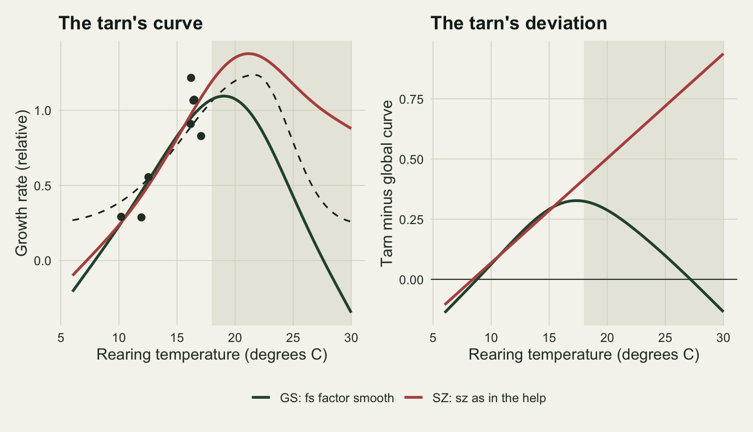

Figure 1: One dataset with the tarn reared only between 6 and 18 degrees. Left: the tarn’s eight animals, its true curve (dashed) and the fits from GS and SZ. Right: the fitted deviation of the tarn from the global curve, the lake level term of each model. The shaded band is the warm half, where the tarn has no animals.

Between 18 and 30 degrees the SZ deviation is a straight line: a least squares line through it leaves residuals below one in ten million, and its slope is 0.043 per degree, carried on unchecked from the cold half. The GS deviation bends back towards zero once the tarn’s animals run out, because its straight line part is penalised like everything else. Against the true curve over the warm half, the root mean squared error of the tarn’s fitted curve was 0.349 for GS, 0.406 for SZ and 0.615 for GI_m2, the other construction with an unpenalised line per lake. G, which gives the tarn no shape of its own, had 0.262. One dataset is one draw; the replication below is what the comparison rests on.

The fit in the figure is the one gam() returns, and for SZ it is not the best fit by the model’s own criterion. The next chunk refits the same dataset with the tarn as the first factor level, once at SZ’s own smoothing parameters, carried over level by level, and once from gam()’s usual start.

wd_first <- wdat; wd_first$pop <- factor(as.character(wdat$pop), levels = first_lev)
nd_first <- new_pop; nd_first$pop <- factor(as.character(new_pop$pop), levels = first_lev)
# smoothing parameters follow the factor levels: global, then one per lake
sp_map   <- wfit$SZ$fit$sp[c(1, n_grp + 1, 2:n_grp)]
same_sp  <- quiet_gam(form_list$SZ, wd_first, sp = sp_map)
order_gap <- max(abs(as.numeric(predict(same_sp, nd_first)) - wfit$SZ$pred))
stopifnot(order_gap < 1e-8)            # the level order does not change the model
w_first  <- fit_model("SZ_first", wdat)
reml_w   <- c(SZ = unname(wfit$SZ$fit$gcv.ubre), first = unname(w_first$fit$gcv.ubre))
tt_first <- predict(w_first$fit, nd_first, type = "terms")
dev_first <- as.numeric(tt_first[tarn_i, grep("pop", colnames(tt_first))[1]])
line_first <- lm(dev_first[warm] ~ grid_t[warm])
stopifnot(max(abs(residuals(line_first))) < 1e-7)
dev_first_slope <- unname(coef(line_first)[2])
warm_first <- sqrt(mean((w_first$pred[tarn_i][warm] - tru_tarn[warm])^2))

At the same smoothing parameters the relabelled fit reproduces SZ’s predictions to rounding error, so the order of the levels is not part of the model. From its own start, though, the optimiser stopped somewhere else: a restricted maximum likelihood score of 7.389 against 9.272 for the fit in the figure (mgcv reports the score as a negative log likelihood, so lower is better). The restricted likelihood of SZ has more than one local maximum, and gam() stopped at a lower one. At the better maximum the tarn’s warm-half deviation is again a straight line to rounding error, with a slope of 0.048 per degree, and the warm-half error is 0.457, against 0.406 for the fit shown. The replication below keeps both fits for SZ.

Forty tarns sampled on the cold half

Each replicate draws six new lakes with the tarn sampled between 6 and 18 degrees, fits all ten models (and SZ once more from the relabelled start), and records for the tarn the root mean squared error of its fitted curve against its true curve over the warm half (the grid from 18.25 to 30 degrees), the same over the cold half, and the error of the fitted optimum; for the five other lakes it records the mean of their errors over the whole range. The same datasets are used for every model, so the comparisons are paired. A control cell repeats four of the models with the tarn sampled over the whole range, 30 datasets drawn from the same seed, so that its first 30 sets of lakes match the first 30 of the cold-half cell.

one_rep <- function(tarn_lo, tarn_hi, models) {
  sim   <- sim_pops(tarn_lo, tarn_hi)
  gi    <- as.integer(new_pop$pop)
  truth <- tpc_true(new_pop$temp, sim$opt[gi], sim$lev[gi])
  do.call(rbind, lapply(models, function(nm) {
    fm   <- fit_model(nm, sim$dat); pred <- fm$pred
    err  <- pred - truth; et <- err[tarn_i]
    data.frame(model = nm, reml = unname(fm$fit$gcv.ubre),
               warm = sqrt(mean(et[grid_t > t_mid]^2)),
               cold = sqrt(mean(et[grid_t < t_mid]^2)),
               opt_err = grid_t[which.max(pred[tarn_i])] - sim$opt[n_grp],
               opt_hat = grid_t[which.max(pred[tarn_i])],
               five = mean(sqrt(tapply(err[!tarn_i]^2, droplevels(new_pop$pop[!tarn_i]), mean))))
  }))
}
run_cell <- function(tarn_lo, tarn_hi, n_data, models, seed = 7171) {
  set.seed(seed)
  cell <- lapply(seq_len(n_data), function(r) cbind(rep = r, one_rep(tarn_lo, tarn_hi, models)))
  cbind(lo = tarn_lo, hi = tarn_hi, do.call(rbind, cell))
}
n_main <- 40; n_side <- 30
fit_models <- names(form_list)
four_models <- c("G", "GS", "SZ", "SZ_m1")
cell_18 <- run_cell(t_lo, t_mid, n_main, fit_models)
all_models <- setdiff(fit_models, "SZ_first")   # SZ_first is a second start for SZ, not a model
cell_30 <- run_cell(t_lo, t_hi, n_side, four_models)

cell_mean <- function(cell, metric, mod) mean(cell[[metric]][cell$model == mod])
cell_se   <- function(cell, metric, mod) {
  x <- cell[[metric]][cell$model == mod]; sd(x) / sqrt(length(x))
}
# paired comparison of two models on the same datasets (by default against GS)
vs_gs <- function(cell, mod, metric = "warm", ref = "GS") {
  a <- cell[cell$model == mod, ]; b <- cell[cell$model == ref, ]
  a <- a[order(a$rep), ]; b <- b[order(b$rep), ]
  d <- a[[metric]] - b[[metric]]
  c(ratio = mean(a[[metric]]) / mean(b[[metric]]), diff = mean(d),
    se = sd(d) / sqrt(length(d)), med_ratio = median(a[[metric]] / b[[metric]]),
    twice = mean(a[[metric]] > 2 * b[[metric]]))
}
m18 <- function(mod, metric = "warm") cell_mean(cell_18, metric, mod)
cmp18 <- sapply(setdiff(all_models, "GS"), function(mod) vs_gs(cell_18, mod))
cold_range <- range(sapply(all_models, m18, metric = "cold"))
opt_mae <- sapply(all_models, function(mod) mean(abs(cell_18$opt_err[cell_18$model == mod])))
five_mean <- sapply(all_models, m18, metric = "five")
stopifnot(names(which.max(sapply(all_models, m18, metric = "cold"))) == "SZ",
          names(which.min(five_mean)) == "SZ_m1")
cmp30 <- sapply(setdiff(four_models, "GS"), function(mod) vs_gs(cell_30, mod))
m30 <- sapply(four_models, function(mod) cell_mean(cell_30, "warm", mod))
worst_m1 <- cell_18[cell_18$model == "SZ_m1", ][which.max(cell_18$warm[cell_18$model == "SZ_m1"]), ]
worst_m1_gs <- cell_18$warm[cell_18$model == "GS" & cell_18$rep == worst_m1$rep]
worst_m1_sz <- cell_18$warm[cell_18$model == "SZ" & cell_18$rep == worst_m1$rep]
# share of SZ's excess over GS that a variant keeps, and SZ against its shared-parameter twin
excess_share <- function(mod) (m18(mod) - m18("GS")) / (m18("SZ") - m18("GS"))
sz_vs_id <- vs_gs(cell_18, "SZ", ref = "SZ_id")
# SZ from two starts: gam()'s own, and the relabelled fit; a lower REML score is better
sz_a <- cell_18[cell_18$model == "SZ", ];       sz_a <- sz_a[order(sz_a$rep), ]
sz_b <- cell_18[cell_18$model == "SZ_first", ]; sz_b <- sz_b[order(sz_b$rep), ]
two_max   <- sum(abs(sz_a$reml - sz_b$reml) > 1e-3)   # starts that stopped at different maxima
b_better  <- sum(sz_b$reml < sz_a$reml - 1e-3)
sz_better <- ifelse(sz_b$reml < sz_a$reml, sz_b$warm, sz_a$warm)
# SZ_m1 without its worst dataset
m1_rows <- cell_18[cell_18$model == "SZ_m1", ]; m1_rows <- m1_rows[order(m1_rows$rep), ]
gs_rows <- cell_18[cell_18$model == "GS", ];    gs_rows <- gs_rows[order(gs_rows$rep), ]
keep_m1 <- m1_rows$rep != worst_m1$rep
m1_ratio_wo <- mean(m1_rows$warm[keep_m1]) / mean(gs_rows$warm[keep_m1])
sz_ts_vs_sel <- vs_gs(cell_18, "SZ_ts", ref = "SZ_sel")

mod_lab <- c(G = "G: global curve, lake intercept", GS = "GS: fs factor smooth",
             GI = "GI: by smooths, m = 1", GI_m2 = "GI_m2: by smooths, m = 2",
             SZ = "SZ: sz as in the help", SZ_m1 = "SZ_m1: sz, m = 1",
             SZ_id = "SZ_id: sz, one smoothing parameter", SZ_sel = "SZ_sel: sz, select = TRUE",
             SZ_ts = "SZ_ts: sz, shrinkage basis",
             G_line = "G_line: global curve, fixed line per lake")
null_kind <- c(G = "nothing", GS = "nothing", GI = "nothing", SZ_sel = "nothing",
               SZ_m1 = "a constant per lake", GI_m2 = "a straight line per lake",
               SZ = "a straight line per lake", SZ_id = "a straight line per lake",
               SZ_ts = "nothing", G_line = "a straight line per lake")
rmse_tab <- rbind(
  data.frame(model = all_models, cell = "Tarn sampled 6 to 18 degrees",
             mean = sapply(all_models, m18),
             se = sapply(all_models, function(mod) cell_se(cell_18, "warm", mod))),
  data.frame(model = four_models, cell = "Tarn sampled 6 to 30 degrees",
             mean = m30,
             se = sapply(four_models, function(mod) cell_se(cell_30, "warm", mod))))
rmse_tab$label <- factor(mod_lab[rmse_tab$model], levels = rev(mod_lab[all_models]))
rmse_tab$kind  <- factor(null_kind[rmse_tab$model],
                         levels = c("nothing", "a constant per lake", "a straight line per lake"))
ggplot(rmse_tab, aes(mean, label, colour = kind)) +
  geom_errorbar(aes(xmin = mean - 2 * se, xmax = mean + 2 * se), orientation = "y",
                width = 0.3, linewidth = 0.5) +
  geom_point(size = 2.8) +
  facet_wrap(~ cell) +
  scale_colour_manual(values = c(te_forest, te_gold, te_rust), name = "Left unpenalised:") +
  labs(x = "Warm-half error of the tarn's curve (RMSE)", y = NULL) +
  guides(colour = guide_legend(title.position = "top", title.hjust = 0.5)) +
  theme_datasheet() + theme(legend.position = "bottom")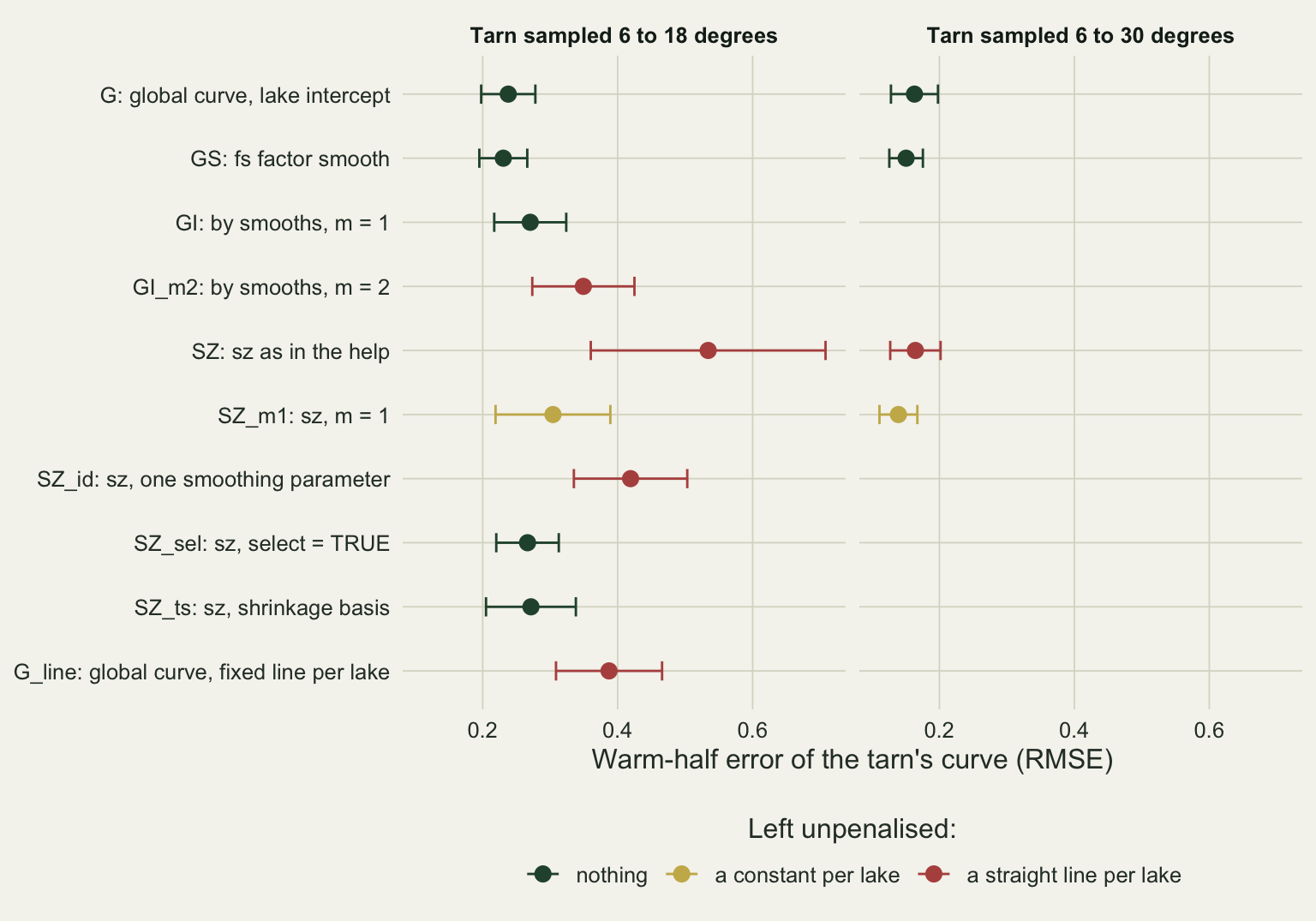

Figure 2: Mean root mean squared error of the tarn’s fitted curve over the warm half (18 to 30 degrees), with the tarn sampled only on the cold half (left, 40 datasets) or over the whole range (right, 30 datasets). Bars are two Monte Carlo standard errors. Colour shows what the lake level term leaves unpenalised.

With the tarn sampled on the cold half, SZ’s error over the warm half averaged 0.534 against 0.231 for GS, a ratio of 2.32 (paired difference 0.304, standard error 0.081). The errors have a long right tail, so the dataset by dataset view matters too: the median of the per-dataset ratio was 1.70, and SZ’s error was more than twice GS’s in 45 per cent of the datasets. G, which does not try to give the tarn a shape, averaged 0.238 (difference from GS 0.007, standard error 0.012). With the tarn sampled over the whole range the gap closes: 0.164 for SZ against 0.151 for GS, a ratio of 1.09, with every model between 0.139 and 0.164. The failure belongs to partial coverage, not to "sz" as such.

The two starts disagreed in the replication too. In 16 of the 40 datasets the fit with the tarn as the first level stopped at a different maximum of the restricted likelihood from gam()’s own fit, and in 9 of those it found the better one. Keeping, in each dataset, whichever of the two fits scored better gave SZ a mean warm-half error of 0.557, 2.42 times GS’s, so choosing the better of the two maxima does not close the gap to GS. The rest of the post reports gam()’s own fits.

Where the tarn has data every construction does well: over the cold half the mean errors ran from 0.066 to 0.092, SZ’s the highest. For the five well sampled lakes the difference was small too, a mean error of 0.126 for SZ and 0.116 for GS. And it carries into the quantity the lakes were reared for: SZ missed the tarn’s optimum by 2.47 degrees on average, GS by 1.64 and G by 1.81.

The variants say which part of SZ does the damage. Fixing the straight line with no penalty at all, G_line, gave 0.387, a ratio of 1.68 to GS, and sharing one smoothing parameter across SZ’s lakes, SZ_id, gave 0.419 (1.82); both keep the line unpenalised, and they carry 52 and 62 per cent of SZ’s excess over GS. GI_m2, the by construction with the same unpenalised line, gave 0.349 (1.51). Whether the separate smoothing parameter for each lake adds the rest is not settled here: SZ was above SZ_id by 0.115, with a standard error of 0.079, which does not separate the two.

Penalising the null space removed most of the excess. With select = TRUE SZ averaged 0.266, a ratio of 1.16 to GS with a paired difference of 0.036 (standard error 0.023) and a median per-dataset ratio of 1.02; 12 per cent of SZ’s excess over GS was left. select = TRUE penalises the global smooth’s null space too. SZ_ts penalises only the lake level term, and it averaged 0.271, a paired difference from SZ_sel of 0.005 (standard error 0.033): the repair sits in the "sz" term. GI, whose m = 1 deviations lose their only unpenalised function to the centring constraint, averaged 0.270 (difference 0.040, standard error 0.022).

Lowering the order on SZ is not the same thing. SZ_m1 averaged 0.304, a ratio of 1.32 to GS (difference 0.074, standard error 0.042). Its median per-dataset ratio was 1.17, well below SZ’s 1.70, but its tail is long: in one dataset its warm-half error was 1.648, where GS had 0.108 and SZ itself 0.136. With m = 1 the straight line is penalised, but each lake keeps its own smoothing parameter. The next chunk refits that one dataset.

set.seed(7171)                                   # the seed of the cold-half cell
for (r in seq_len(worst_m1$rep)) w_sim <- sim_pops(t_lo, t_mid)
w_truth <- tpc_true(grid_t, w_sim$opt[n_grp], w_sim$lev[n_grp])
m1_fit  <- fit_model("SZ_m1", w_sim$dat)
warm_err <- function(pred) sqrt(mean((pred[tarn_i][warm] - w_truth[warm])^2))
stopifnot(abs(warm_err(m1_fit$pred) - worst_m1$warm) < 1e-8)   # the same fit as in the cell
tarn_sp_m1 <- unname(m1_fit$fit$sp[n_grp + 1])                # the tarn's smoothing parameter
stopifnot(tarn_sp_m1 < 1e-3)
at_24 <- grid_t == 24
m1_24 <- m1_fit$pred[tarn_i][at_24]; true_24 <- w_truth[at_24]
m1_id <- quiet_gam(growth ~ s(temp, k = k_basis, m = 2) +
                     s(pop, temp, bs = "sz", k = k_basis, m = 1, id = 1), w_sim$dat)
warm_m1_id <- warm_err(as.numeric(predict(m1_id, new_pop)))

In that dataset the restricted likelihood gave the tarn a smoothing parameter of practically zero, so its deviation was free to follow its eight cold animals and swung away beyond them: the tarn’s curve stood at -1.46 at 24 degrees, where the truth is 0.61. With one smoothing parameter shared across the lakes (id = 1) the same data gave a warm-half error of 0.228, so most of that failure came from the tarn’s own smoothing parameter. On the five well sampled lakes SZ_m1 had the lowest mean error of all, 0.100, and it did not fall behind GS with the tarn sampled over the whole range either (0.139 against 0.151).

pair_mods <- c("SZ", "SZ_m1", "SZ_sel", "G")
gs_warm <- cell_18[cell_18$model == "GS", c("rep", "warm")]
pairs_df <- do.call(rbind, lapply(pair_mods, function(mod) {
  a <- cell_18[cell_18$model == mod, c("rep", "warm")]
  data.frame(model = mod, gs = gs_warm$warm[match(a$rep, gs_warm$rep)], alt = a$warm)
}))
pairs_df$model <- factor(pairs_df$model, levels = pair_mods,
                         labels = c("SZ: sz as in the help", "SZ_m1: sz, m = 1",
                                    "SZ_sel: sz, select = TRUE", "G: no lake shape"))
ggplot(pairs_df, aes(gs, alt)) +
  geom_abline(slope = 1, intercept = 0, colour = te_body, linetype = "dashed", linewidth = 0.4) +
  geom_point(colour = te_rust, alpha = 0.75, size = 1.8) +
  facet_wrap(~ model, nrow = 1) +
  scale_x_log10() + scale_y_log10() +
  labs(x = "Warm-half error under GS (log scale)", y = "Warm-half error, construction (log scale)") +
  theme_datasheet()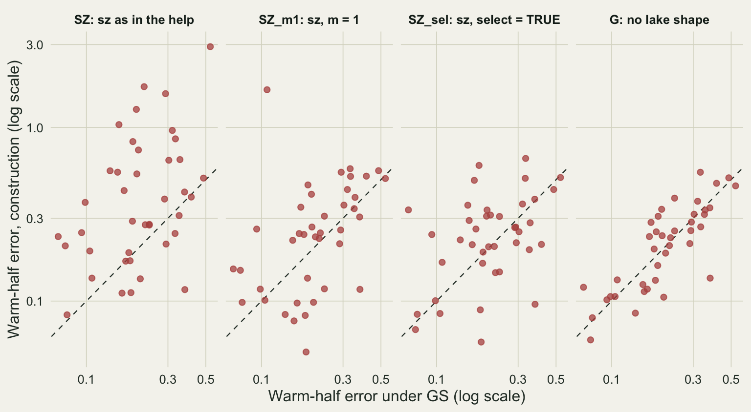

Figure 3: Each point is one of the 40 datasets with the tarn sampled on the cold half: the tarn’s warm-half error under a construction against the same dataset’s error under GS. Points above the dashed line are datasets in which the construction did worse than GS.

A straight line through eight animals

How large an error should an unpenalised line give? A least squares line through 8 points with noise standard deviation \(\sigma\) has prediction variance \(\sigma^2\{1/n + (t - \bar x)^2 / S_{xx}\}\) at temperature \(t\). Plugging in the population values for eight temperatures spread evenly between 6 and 18 degrees, and averaging over the warm-half grid, gives the error the line would have from noise alone, even if the tarn’s true deviation from the global curve were zero everywhere. The chunk computes that plug-in value and the same error averaged over many random sets of eight temperatures drawn on the cold half (the squared error is averaged over the sets before the square root is taken, so it is a root mean square, like the errors above).

g_warm <- grid_t[grid_t > t_mid]
sd_u   <- (t_mid - t_lo) / sqrt(12)                 # sd of a uniform on the cold half
centre <- (t_lo + t_mid) / 2
line_plug <- sqrt(sd_eps^2 / n_sparse + sd_eps^2 / (n_sparse * sd_u^2) * mean((g_warm - centre)^2))
set.seed(7180)
n_design <- 20000
xs   <- matrix(runif(n_design * n_sparse, t_lo, t_mid), n_design)
xbar <- rowMeans(xs)
sxx  <- rowSums((xs - xbar)^2)
msd  <- rowMeans(outer(xbar, g_warm, function(a, b) (b - a)^2))
line_exact <- sqrt(mean(sd_eps^2 * (1 / n_sparse + msd / sxx)))   # root of the mean over designs

The plug-in value is 0.200 and the average over 20000 random sets of temperatures 0.235, larger because a random set of eight temperatures sometimes bunches and leaves the slope poorly pinned. That is the price of noise alone, in a straight line fitted to the tarn’s own animals and carried across twelve degrees. It is the same size as G’s whole warm-half error, 0.238, which comes from the part of the tarn’s true deviation that eight cold animals cannot reveal. G_line, which is the global curve plus exactly such a line for every lake, averaged 0.387; the constructions that penalise the line stayed near G.

How much of the range is missing

The cold half is one point on a scale. The next chunk moves the tarn’s upper limit to 12 and 24 degrees, 30 datasets each from the same seed, with the four models that frame the result; the error is still measured over 18 to 30 degrees, so at 12 the gap starts six degrees before the measured stretch and at 24 half of the stretch has data. It also turns the design over: the tarn sampled only between 18 and 30 degrees, with its optimum inside the data, and the error measured over the cold half it did not see.

sweep_models <- four_models
cell_12  <- run_cell(t_lo, 12, n_side, sweep_models)
cell_24  <- run_cell(t_lo, 24, n_side, sweep_models)
cell_mir <- run_cell(t_mid, t_hi, n_side, sweep_models)

sweep_tab <- do.call(rbind, lapply(list(cell_12, cell_18, cell_24, cell_30), function(cl) {
  data.frame(cap = cl$hi[1], model = sweep_models,
             mean = sapply(sweep_models, function(mod) cell_mean(cl, "warm", mod)),
             se = sapply(sweep_models, function(mod) cell_se(cl, "warm", mod)))
}))
cmp12 <- sapply(c("G", "SZ", "SZ_m1"), function(mod) vs_gs(cell_12, mod))
cmp24 <- sapply(c("G", "SZ", "SZ_m1"), function(mod) vs_gs(cell_24, mod))
cmp_mir <- sapply(c("G", "SZ", "SZ_m1"), function(mod) vs_gs(cell_mir, mod, "cold"))
mir_mean <- sapply(sweep_models, function(mod) cell_mean(cell_mir, "cold", mod))
mir_opt  <- sapply(sweep_models, function(mod) mean(abs(cell_mir$opt_err[cell_mir$model == mod])))
mir_cold_edge <- sapply(sweep_models, function(mod) mean(cell_mir$opt_hat[cell_mir$model == mod] == t_lo))

sweep_tab$model <- factor(mod_lab[sweep_tab$model], levels = mod_lab[sweep_models])
ggplot(sweep_tab, aes(cap, mean, colour = model, linetype = model, shape = model)) +
  geom_errorbar(aes(ymin = mean - 2 * se, ymax = mean + 2 * se), width = 0.6, linewidth = 0.45,
                linetype = "solid", position = position_dodge(width = 1.2)) +
  geom_line(linewidth = 0.9, position = position_dodge(width = 1.2)) +
  geom_point(size = 2.4, position = position_dodge(width = 1.2)) +
  scale_colour_manual(values = c(te_forest, te_forest, te_rust, te_gold), name = NULL) +
  scale_linetype_manual(values = c("22", "solid", "solid", "solid"), name = NULL) +
  scale_shape_manual(values = c(1, 16, 16, 16), name = NULL) +
  scale_x_continuous(breaks = c(12, 18, 24, 30)) +
  labs(x = "Warmest temperature at which the tarn was reared (degrees C)",
       y = "Warm-half error of the tarn's curve (RMSE)") +
  guides(colour = guide_legend(nrow = 2), linetype = guide_legend(nrow = 2), shape = guide_legend(nrow = 2)) +
  theme_datasheet() + theme(legend.position = "bottom", legend.key.width = unit(2.4, "lines"))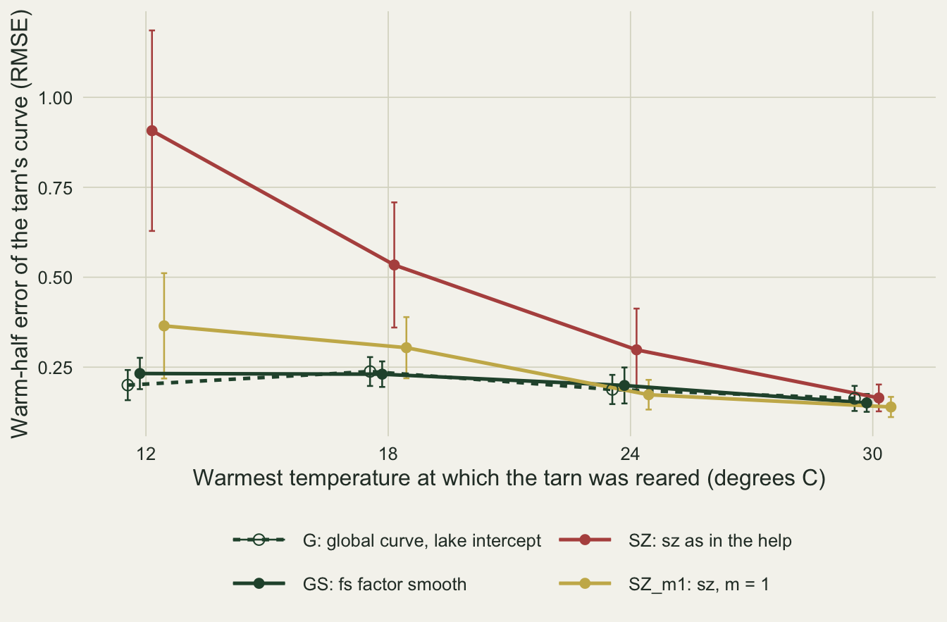

Figure 4: Mean warm-half error of the tarn’s curve against the upper limit of the tarn’s rearing temperatures, for four constructions. The point at 18 degrees uses the 40 datasets above, the others 30 datasets each. Bars are two Monte Carlo standard errors. Colours follow the dot plot of warm-half errors above: green leaves nothing unpenalised, gold a constant per lake, rust a straight line per lake.

The shorter the tarn’s range, the worse SZ does against GS: a ratio of 3.90 with the tarn stopping at 12 degrees (SZ 0.907, GS 0.232), 2.32 at 18, 1.50 at 24 and 1.09 over the whole range. SZ_m1 gets worse at the short end: its ratio to GS was 1.57 at 12 degrees (median per-dataset ratio 1.20), against 0.87 at 24. G stays with GS throughout (0.86 at 12 degrees, 0.94 at 24).

Turning the design over does not rescue SZ. With the tarn reared only between 18 and 30 degrees, so that its optimum lies inside its data, the error over the unseen cold half was 0.482 for SZ against 0.198 for GS, a ratio of 2.43 (difference 0.284, standard error 0.061). The ratio was 1.21 for SZ_m1 (median per-dataset ratio 1.10) and 1.00 for G. Having the optimum in the data did not protect the optimum either: SZ missed it by 3.36 degrees on average against 1.39 for GS. In 10 per cent of the SZ fits the highest point of the tarn’s curve sat at 6 degrees, the cold edge of the range and at least twelve degrees from the nearest animal, against 0 per cent for GS.

What to report

Report the temperature range, or the range of whatever covariate the smooth runs along, for every group, next to that group’s curve. A group whose data cover only part of the range is a different case from a group with few data, and the hierarchical structure does not treat the two alike.

When groups cover different parts of the range, do not take "sz" with its defaults. Here it left a straight line per lake unpenalised and a smoothing parameter per lake, and the half-sampled tarn’s warm half came out 2.32 times as wrong as under the "fs" factor smooth. GS and G did equally well in the missing half, and "sz" with its null space penalised, by select = TRUE or by the shrinkage basis, came close to them. Lowering the penalty order to one helped on average but left a long tail and did not hold when the tarn’s range was shorter, so it is not a repair to rely on.

Plot each group’s deviation term over the full range with predict(..., type = "terms"). A deviation that runs out of the group’s data as a straight line, as SZ’s did in the worked example, is the signature of an unpenalised null space, and it is visible before any comparison with a truth.

Say what the curve means where the group has no data. Even the best constructions here did no better than G, which gives the tarn the global shape plus an offset. Beyond its data the tarn’s curve is the global curve’s assumption, not an estimate for the tarn, and an optimum or a thermal limit read off that stretch should be reported as such.

Honest limits

The truth is the one the hierarchical models are built for: every lake shares the curve’s shape and differs by its optimum and offset. A tarn with a genuinely different warm limb, for example a steeper fall, is exactly what a penalised deviation shrinks away and what an unpenalised line might partly follow; that case was not simulated, so the cost of select = TRUE or of GS when a half-sampled group really is different is not measured here.

The design is one point: six lakes, twelve animals in five and eight in the tarn, a Gaussian response, k = 6, REML. Only one group is half-sampled. The partly sampled groups of real studies are often several, and with more of them the global curve itself would be pulled; that was not tried. Every construction was fitted from gam()’s own start, and SZ from one more. The constructions that give each lake its own smoothing parameter can have several maxima of the restricted likelihood, as SZ did, and they were not searched from more starts, so their errors in single datasets depend on which maximum the optimiser reaches.

Replication is 40 datasets in the main cell and 30 in each of the others. The errors are skewed, so means carry wide Monte Carlo standard errors and are given with medians; the mean of SZ_m1 with the tarn stopping at 18 degrees leans on a single dataset: without it, its ratio to GS falls from 1.32 to 1.15. Its median ratio to GS was above one there and at 12 degrees as well, so the verdict against it does not rest on that dataset alone. GI, GI_m2, the select = TRUE refit and the G_line, SZ_id and SZ_ts variants were run only with the tarn on the cold half.

Only point estimates were scored. Whether the confidence band of each construction widens enough over the missing half to cover the truth, which is what a reader would lean on, was not measured.

References

Marra G, Wood SN 2011 Computational Statistics and Data Analysis 55(7):2372-2387 (10.1016/j.csda.2011.02.004)

Pedersen EJ, Miller DL, Simpson GL, Ross N 2019 PeerJ 7:e6876 (10.7717/peerj.6876)

Wood SN 2011 Journal of the Royal Statistical Society Series B 73(1):3-36 (10.1111/j.1467-9868.2010.00749.x)

Wood SN 2017 Generalized Additive Models: An Introduction with R, 2nd edition (ISBN 978-1-4987-2833-1)

Related tutorials

• Hierarchical GAMs and factor smooths in mgcv
• Checking a generalised additive model
• Choosing the basis dimension k in mgcv
• Penalised regression splines from scratch