library(ggplot2)
library(patchwork)

te_paper  <- "#f5f4ee"
te_ink    <- "#16241d"
te_body   <- "#2c3a31"
te_forest <- "#275139"
te_rust   <- "#b5534e"
te_gold   <- "#c9b458"
te_line   <- "#dad9ca"

theme_datasheet <- function() {
  theme_minimal(base_size = 12) +
    theme(plot.background  = element_rect(fill = te_paper, colour = NA),
          panel.background = element_rect(fill = te_paper, colour = NA),
          panel.grid.major = element_line(colour = te_line, linewidth = 0.3),
          panel.grid.minor = element_blank(),
          text             = element_text(colour = te_body),
          plot.title       = element_text(colour = te_ink, face = "bold"),
          plot.subtitle    = element_text(colour = te_body),
          axis.text        = element_text(colour = te_body))
}Drone flushing pushes a survey count both ways
R
drones
survey design
simulation
monitoring
ecology tutorial
Simulating a lawnmower drone survey in R: flushing recounts animals that fly into the not yet imaged strip, and loses the ones driven off the block edge.
A drone flies a gull colony on a shallow lagoon. The flight plan is the ordinary one: a rectangular block, parallel strips, back and forth, nadir camera, one image every second. The birds are not indifferent to it. Some of them lift off when the aircraft is still fifty metres away, fly a short distance, and settle again. The pilot knows this is a welfare question. What is less often asked is what it does to the number at the bottom of the count sheet.
The usual worry about a photographic mosaic is double counting, and the usual fix is a matching rule: two images that show the same animal must be reconciled, by overlap geometry or by appearance. That worry treats the animals as fixed and the images as the problem. This post treats the images as exact and the animals as the problem. Every individual in the block is imaged whenever the nadir line passes over it, with no missed detections and no identification error at all, and the count still comes out wrong, because the survey moved the animals while it was counting them.
The direction it comes out wrong is the part that is hard to guess. This post finds two carriers with opposite signs. An animal that flies sideways out of ground the drone has already imaged and into ground it has not yet reached is counted a second time, which inflates the total. An animal that is flushed again and again as the aircraft works across the block drifts over the boundary and is lost, which deflates it. Which carrier wins is set by the flush radius and, more sharply, by whether the block has an edge the animals can leave through. The deduplication literature asks whether two images show one animal; this post asks what the drone did to the animal between the two images, and finds that at the flush radii a low multirotor provokes in waterbirds and seals, 30 to 60 m, a fenced block can only inflate the count, while on an open block most of the undercount, though not all of it, is an animal that left.
Responsive movement is not a new subject in survey statistics. Turnock and Quinn set out in 1991 what animals moving in response to an approaching observer do to a line transect estimate, Buckland and Turnock proposed a two-observer design that measures it, and Glennie, Buckland and Thomas quantified how ordinary movement inflates line transect encounter rates. In all of that work the displacement matters because it changes the perpendicular distance that gets recorded, which is the quantity the detection function is fitted to. A mosaic has no perpendicular distance. Displacement matters here for a different reason: it changes whether the animal is standing on ground that has been imaged or on ground that has not. The drone disturbance literature, reviewed by Mulero-Pazmany and colleagues and by Hodgson and Koh, measures flight initiation distances and stress responses without attaching a count bias to them, and Brack, Kindel and Oliveira set out the detection errors in aerial image surveys without this one. That gap is what the simulation below fills.
Three posts on this site sit next to the problem and stop short of it. Line transects along tracks and avoidance ends its honest limits by saying that responsive movement away from an approaching observer is a different process from the static avoidance gradient it simulates; this post is that different process, in mosaic geometry rather than in distance sampling. Pitfall catches and the depletion zone has a survey device that removes animals from a random walk, but a pitfall is a passive sink that sits still and waits, and a drone is a plough that sweeps the whole block in one direction. Identification errors in capture-recapture finds a pair of opposed errors whose rates can be tuned until they cancel; here the two errors are not rates but mechanisms, and what balances them is a design parameter and the presence or absence of a boundary.
The block, the flight and the counting rule
The design constants were fixed before anything ran and none of them was changed afterwards. The block is 800 m square. The drone flies ten strips of 80 m at 10 m/s, back and forth, in steps of one second. Three hundred animals start uniformly in the block. An animal is recorded once every time the nadir line crosses its along-track position while it is laterally inside the strip being flown. That is a crossing rule: the signed offset between the drone and the animal along the flight direction has to change sign within one step. The weaker alternative, recording an animal whenever it is inside the ten metre interval the camera swept during that second, counts an animal running ahead of the aircraft at 3 m/s twice in consecutive seconds, which is an artefact of the rule and not of the survey.
A flushed animal runs directly away from the drone at 3 m/s for a fixed distance, with a heading error of 30 degrees, then rests. It can be flushed again. The two parameters that describe the response are the flush radius, the distance at which the aircraft provokes a flight, and the flush distance, how far the animal goes.
The block edge is either open or sealed, and what those two words do in the code decides most of what follows. An open edge is permeable rather than absorbing: an animal that crosses it is outside the imaged area and stops being counted there, but it is still walking, and if a later flush carries it back inside it is counted again. A sealed edge is a shore, and a bird that is still in flight when it reaches the water has to do something, so two versions of it are run. Under the bouncing rule the position is mirrored back into the block and the outward component of the heading is reversed, which is the textbook reflecting boundary: the rest of the flight is spent travelling away from the wall. Under the stopping rule the position is clamped to the boundary and the flight ends there, which is the more literal reading of a colony on an island or a haulout ringed by water. Mirroring the position and leaving the heading alone, the version that is easiest to write, is neither: it holds a still flying bird against the wall for the rest of its flight, and the honest limits section at the end returns to what that does.
block_m   <- 800
strip_m   <- 80
v_drone   <- 10
v_animal  <- 3
n_block   <- 300
head_base <- pi / 6
shore_eps <- 1e-6

make_path <- function(buf) {
  lo <- -buf
  hi <- block_m + buf
  n_strip <- (hi - lo) / strip_m
  xs <- seq(lo, hi, by = v_drone)
  do.call(rbind, lapply(seq_len(n_strip), function(s) {
    cbind(x = if (s %% 2 == 1) xs else rev(xs),
          y = lo + (s - 0.5) * strip_m, s = s)
  }))
}

fly_block <- function(n_animal, r_f, d_f = 100, pf = 1, head_sd = head_base,
                      edge = "open", along_only = FALSE, walk_sd = 0,
                      buf = 0, refuge = NA, surround = 0, keep_track = FALSE) {
  path    <- make_path(buf)
  n_step  <- nrow(path)
  n_strip <- max(path[, "s"])
  lo <- -buf
  hi <- block_m + buf
  ax <- runif(n_animal, 0, block_m)
  ay <- runif(n_animal, 0, block_m)
  if (surround > 0) {
    ring_area <- (block_m + 2 * surround)^2 - block_m^2
    n_ring <- rpois(1, n_animal / block_m^2 * ring_area)
    cand_x <- runif(4 * n_ring, -surround, block_m + surround)
    cand_y <- runif(4 * n_ring, -surround, block_m + surround)
    outside <- which(cand_x < 0 | cand_x > block_m |
                       cand_y < 0 | cand_y > block_m)[seq_len(n_ring)]
    ax <- c(ax, cand_x[outside])
    ay <- c(ay, cand_y[outside])
  }
  n_tot <- length(ax)
  core <- seq_len(n_animal)
  togo <- rep(0, n_tot)
  ux <- uy <- numeric(n_tot)
  seen <- integer(n_tot)
  ever_out <- logical(n_tot)
  per_strip <- integer(n_strip)
  rel_prev <- path[1, "x"] - ax
  n_flush <- 0
  n_moving <- 0
  trk <- if (keep_track) matrix(NA_real_, n_step, 2 * n_tot) else NULL
  for (k in 2:n_step) {
    dx <- path[k, "x"]
    dy <- path[k, "y"]
    s_now <- path[k, "s"]
    if (walk_sd > 0) {
      ax <- ax + rnorm(n_tot, 0, walk_sd)
      ay <- ay + rnorm(n_tot, 0, walk_sd)
    }
    if (r_f > 0) {
      near <- which(sqrt((ax - dx)^2 + (ay - dy)^2) < r_f & togo <= 0 &
                      runif(n_tot) < pf)
      if (length(near)) {
        ang <- atan2(ay[near] - dy, ax[near] - dx)
        if (along_only) ang <- ifelse(cos(ang) >= 0, 0, pi)
        if (!is.na(refuge)) ang <- rep(refuge, length(near))
        ang <- ang + rnorm(length(near), 0, head_sd)
        ux[near] <- cos(ang)
        uy[near] <- sin(ang)
        togo[near] <- d_f
        n_flush <- n_flush + length(near)
      }
      moving <- which(togo > 0)
      if (length(moving)) {
        step_m <- pmin(v_animal, togo[moving])
        ax[moving] <- ax[moving] + ux[moving] * step_m
        ay[moving] <- ay[moving] + uy[moving] * step_m
        togo[moving] <- togo[moving] - step_m
        n_moving <- n_moving + length(moving)
      }
    }
    if (edge != "open") {
      past_lo_x <- ax < lo; past_hi_x <- ax > hi
      past_lo_y <- ay < lo; past_hi_y <- ay > hi
      if (edge == "bounce") {
        ax <- ifelse(past_lo_x, 2 * lo - ax, ifelse(past_hi_x, 2 * hi - ax, ax))
        ay <- ifelse(past_lo_y, 2 * lo - ay, ifelse(past_hi_y, 2 * hi - ay, ay))
        turn_x <- past_lo_x | past_hi_x
        turn_y <- past_lo_y | past_hi_y
        ux[turn_x] <- -ux[turn_x]
        uy[turn_y] <- -uy[turn_y]
      } else {
        ax <- pmin(pmax(ax, lo + shore_eps), hi - shore_eps)
        ay <- pmin(pmax(ay, lo + shore_eps), hi - shore_eps)
        togo[past_lo_x | past_hi_x | past_lo_y | past_hi_y] <- 0
      }
    }
    ever_out <- ever_out | !(ax >= lo & ax <= hi & ay >= lo & ay <= hi)
    rel <- dx - ax
    if (path[k - 1, "s"] == s_now) {
      hit <- which(abs(ay - dy) < strip_m / 2 & rel_prev * rel <= 0 &
                     rel != rel_prev)
      seen[hit] <- seen[hit] + 1L
      per_strip[s_now] <- per_strip[s_now] + length(hit)
    }
    rel_prev <- rel
    if (keep_track) trk[k, ] <- c(ax, ay)
  }
  gone <- !(ax >= lo & ax <= hi & ay >= lo & ay <= hi)
  list(stats = c(ratio = sum(seen) / n_animal,
                 twice = mean(seen[core] >= 2),
                 never = mean(seen[core] == 0),
                 out = mean(gone[core]),
                 stayed = mean(seen[core] == 0 & !ever_out[core]),
                 moving = n_moving / (n_animal * (n_step - 1)),
                 flushes = n_flush / n_animal),
       strip = per_strip, seen = seen, track = trk, path = path)
}

run_cell <- function(reps, ...) {
  runs <- lapply(seq_len(reps), function(i) fly_block(n_animal = n_block, ...))
  st <- vapply(runs, function(z) z$stats, numeric(7))
  sp <- vapply(runs, function(z) z$strip, numeric(length(runs[[1]]$strip)))
  list(mean = rowMeans(st), se = apply(st, 1, sd) / sqrt(reps),
       strip = rowMeans(sp), reps = reps)
}
n_rep_main <- 40
n_rep_side <- 25
n_rep_buf <- 20
set.seed(51101)
static_cell <- run_cell(5, r_f = 0)
static_ratio <- static_cell$mean[["ratio"]]
static_twice <- static_cell$mean[["twice"]]
flight_min <- (nrow(make_path(0)) - 1) / 60The rule has one check that has to pass exactly rather than approximately. With no movement at all, every animal is crossed by the nadir line of its own strip once and by no other, so the count divided by the number present must be one and the share counted twice must be zero. It is: 1.000 and 0.000 over five replicate surveys, with the flight lasting 13.5 minutes.
set.seed(51102)
demo <- fly_block(n_animal = 60, r_f = 60, keep_track = TRUE)
demo_path <- as.data.frame(demo$path)
pick_class <- function(code, want) {
  idx <- which(demo$seen == code)
  head(idx, want)
}
show_idx <- c(pick_class(1, 3), pick_class(2, 3), pick_class(0, 3))
lab_of <- c("never counted", "counted once", "counted twice or more")
trk_df <- do.call(rbind, lapply(show_idx, function(i) {
  ok <- !is.na(demo$track[, i])
  data.frame(x = demo$track[ok, i], y = demo$track[ok, 60 + i],
             id = i, cls = lab_of[min(demo$seen[i], 2) + 1])
}))
ends_df <- do.call(rbind, lapply(split(trk_df, trk_df$id), function(z) {
  data.frame(x0 = z$x[1], y0 = z$y[1], x1 = z$x[nrow(z)], y1 = z$y[nrow(z)],
             cls = z$cls[1])
}))
cls_col <- c("never counted" = te_gold, "counted once" = te_forest,
             "counted twice or more" = te_rust)

ggplot() +
  geom_path(data = demo_path, aes(x, y), colour = te_body, alpha = 0.3,
            linewidth = 0.45) +
  annotate("rect", xmin = 0, xmax = block_m, ymin = 0, ymax = block_m,
           fill = NA, colour = te_body, linetype = "dashed", linewidth = 0.4) +
  geom_path(data = trk_df, aes(x, y, group = id, colour = cls),
            linewidth = 0.7) +
  geom_point(data = ends_df, aes(x0, y0, colour = cls), shape = 21,
             fill = te_paper, size = 2) +
  geom_point(data = ends_df, aes(x1, y1, colour = cls), size = 1.8) +
  scale_colour_manual(values = cls_col, name = NULL) +
  coord_equal() +
  labs(x = "along the flight lines (m)", y = "across the flight lines (m)",
       title = "What the survey does to nine of the animals",
       subtitle = "open circle: position at take-off; grey: the drone path") +
  theme_datasheet() +
  theme(legend.position = "bottom", panel.grid.major = element_blank())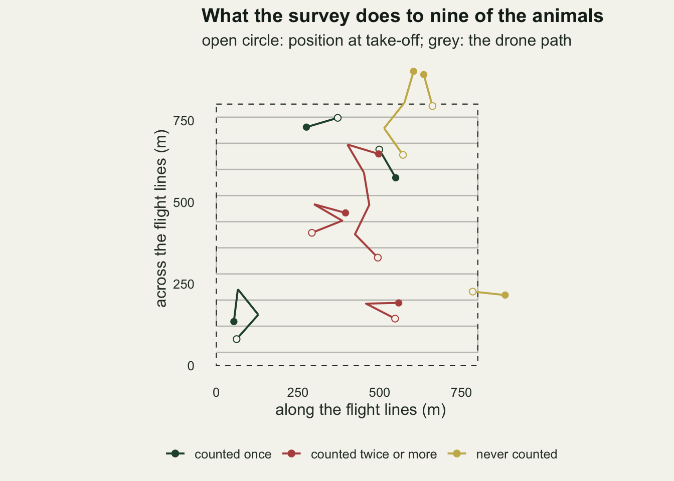
Random movement on its own does not bias the count
Before any flushing, the baseline has to be established, and it is an identity rather than a result. If animals move but their movement has nothing to do with the aircraft, then at the moment each strip is flown the animals are distributed over the block exactly as they were at the start, because nothing has picked a direction. The expected count is the number present. Double counts and misses both occur, and they cancel in expectation. This is worth simulating only because it is the yardstick everything else is measured against, and because the cancellation is easy to disbelieve.
set.seed(51103)
walk_cells <- list(
  `sd 1, sealed edge` = run_cell(n_rep_main, r_f = 0, walk_sd = 1, edge = "bounce"),
  `sd 2, sealed edge` = run_cell(n_rep_main, r_f = 0, walk_sd = 2, edge = "bounce"),
  `sd 1, open edge`   = run_cell(n_rep_main, r_f = 0, walk_sd = 1),
  `sd 2, open edge`   = run_cell(n_rep_main, r_f = 0, walk_sd = 2))
walk_tab <- do.call(rbind, lapply(names(walk_cells), function(nm) {
  cc <- walk_cells[[nm]]
  data.frame(arm = nm, ratio = cc$mean[["ratio"]], se = cc$se[["ratio"]],
             twice = cc$mean[["twice"]], never = cc$mean[["never"]],
             out = cc$mean[["out"]])
}))
walk_fast <- 2
walk_seal <- walk_tab[walk_tab$arm == "sd 2, sealed edge", ]
walk_open <- walk_tab[walk_tab$arm == "sd 2, open edge", ]
walk_dev  <- abs(walk_seal$ratio - 1) / walk_seal$se
sur_m <- 250
set.seed(51109)
sur_walk <- run_cell(n_rep_side, r_f = 0, walk_sd = walk_fast, surround = sur_m)
sur_walk_ratio <- sur_walk$mean[["ratio"]]
sur_walk_se <- sur_walk$se[["ratio"]]
A random walk of 2 m per second in each coordinate, which over the length of the flight displaces an animal by about 57 m in each direction, leaves the count at 0.999 per animal present inside a sealed block, with a Monte Carlo standard error of 0.003 over 40 replicate surveys. That is 0.2 standard errors from one. It gets there by cancellation and not by nothing happening: 0.073 of the animals are counted twice or more and 0.074 are never counted at all.
Open the edge and the same walk gives 0.934, with 0.112 of the animals outside the block when the flight ends. That shortfall is emigration with nothing coming the other way, because the simulation fills the block and leaves the ground around it empty. Repeat the arm with the surrounding landscape populated at the same density out to 250 m, still dividing the count by the animals that were inside the block at take-off, and the count comes to 1.000 with a Monte Carlo standard error of 0.006. A real open boundary carries traffic both ways, and undirected movement across it does not bias the count at all. The 0.934 belongs to the boundary condition rather than to the survey. Both numbers matter later, because the flushing arms are run under exactly the same conditions and are read against them.
Flushing, and a count that changes sign
Now the aircraft provokes the movement. The flush radius runs from zero to 180 m with the flush distance held at 100 m, the response probability at one, and the heading error at 30 degrees. The same grid is run three times: once with an open block edge, and twice with a sealed one, under the two shore rules set out above.
rf_grid <- c(0, 30, 60, 90, 120, 180)
set.seed(51104)
open_cells <- lapply(rf_grid, function(rf) run_cell(n_rep_main, r_f = rf))
refl_cells <- lapply(rf_grid, function(rf) run_cell(n_rep_main, r_f = rf,
                                                    edge = "bounce"))
stop_cells <- lapply(rf_grid, function(rf) run_cell(n_rep_main, r_f = rf,
                                                    edge = "stop"))
as_tab <- function(cells, lab) {
  do.call(rbind, Map(function(rf, cc) {
    data.frame(r_f = rf, edge = lab, ratio = cc$mean[["ratio"]],
               se = cc$se[["ratio"]], twice = cc$mean[["twice"]],
               never = cc$mean[["never"]], out = cc$mean[["out"]],
               stayed = cc$mean[["stayed"]], moving = cc$mean[["moving"]],
               flushes = cc$mean[["flushes"]],
               last_first = cc$strip[length(cc$strip)] / cc$strip[1])
  }, rf_grid, cells))
}
lab_open <- "open edge"
lab_refl <- "sealed: bounced back"
lab_stop <- "sealed: stopped at the shore"
open_tab <- as_tab(open_cells, lab_open)
refl_tab <- as_tab(refl_cells, lab_refl)
stop_tab <- as_tab(stop_cells, lab_stop)
sweep_tab <- rbind(open_tab, refl_tab, stop_tab)
pick <- function(tab, rf) tab[tab$r_f == rf, ]
o30 <- pick(open_tab, 30); o60 <- pick(open_tab, 60); o90 <- pick(open_tab, 90)
o120 <- pick(open_tab, 120); o180 <- pick(open_tab, 180)
r30 <- pick(refl_tab, 30); r60 <- pick(refl_tab, 60); r90 <- pick(refl_tab, 90)
r120 <- pick(refl_tab, 120); r180 <- pick(refl_tab, 180)
s30 <- pick(stop_tab, 30); s60 <- pick(stop_tab, 60); s90 <- pick(stop_tab, 90)
s120 <- pick(stop_tab, 120); s180 <- pick(stop_tab, 180)
se_worst <- max(sweep_tab$se)
cross_rf <- approx(open_tab$ratio[-1], open_tab$r_f[-1], xout = 1)$y
seal_tab <- rbind(refl_tab, stop_tab)
seal_low <- seal_tab[seal_tab$r_f %in% c(30, 60), ]
seal_low_min <- min(seal_low$ratio)
seal_high <- seal_tab[seal_tab$r_f %in% c(120, 180), ]
seal_high_min <- min(seal_high$ratio)
seal_gap <- max(abs(refl_tab$ratio - stop_tab$ratio))
seal_gap_rf <- refl_tab$r_f[which.max(abs(refl_tab$ratio - stop_tab$ratio))]
open_max_never <- max(open_tab$never)
refl_max_never <- max(refl_tab$never)
seal_max_never <- max(seal_tab$never)
seal_gap_low <- max(abs(refl_tab$ratio - stop_tab$ratio)[refl_tab$r_f %in%
                                                         c(30, 60, 90)])
seal_high_dev <- max(abs(seal_high$ratio - 1))
o120_share_stayed <- o120$stayed / o120$never
seal_low_worst <- seal_low[which.min(seal_low$ratio), ]
seal_low_sig <- (seal_low_worst$ratio - 1) / seal_low_worst$se
set.seed(51110)
sur_flush <- run_cell(n_rep_side, r_f = 120, surround = sur_m)
sur_flush_ratio <- sur_flush$mean[["ratio"]]
sur_flush_se <- sur_flush$se[["ratio"]]
On an open block the count per animal present is 1.28 at a flush radius of 30 m, 1.10 at 60 m, 0.92 at 90 m, 0.66 at 120 m and 0.32 at 180 m. The largest Monte Carlo standard error anywhere in the sweep is 0.006, so the differences between those cells are far larger than the simulation noise. The curve crosses one at a flush radius of about 77 m. A survey whose birds lift at 30 m overcounts by more than a quarter; the same survey on a species that lifts at 120 m returns two thirds of the population, and at 180 m under a third of it.
One objection has to be dealt with before the open numbers are read, because the arm fills the block and leaves the ground around it empty, exactly as the walk arm did. Running the 120 m cell again with the surrounding landscape populated to 250 m at the same density, and the count still divided by the animals inside the block at take-off, gives 0.655 with a Monte Carlo standard error of 0.008, against 0.66 with the surround empty. Unlike the walk deficit, the flushing deficit is not a bookkeeping artefact of where the animals were placed. The aircraft pushes animals out of the block and never pushes any in, so immigration does not refill it.
The sealed block separates the two carriers, and it also shows where the answer stops being a property of the flushing and starts being a property of the shore. With the identical flushing dynamics and a boundary the animals cannot cross, the bouncing rule gives 1.29 at 30 m, 1.20 at 60 m, 1.13 at 90 m, 0.97 at 120 m and 0.96 at 180 m, and the stopping rule gives 1.28, 1.19, 1.13, 1.02 and 1.12. The two rules agree where the flush radius is small and part company where it is large: the lowest of the four cells at 30 and 60 m is 1.19, which is 53 Monte Carlo standard errors above one, while at 120 and 180 m the lowest is 0.96 and the two rules differ from each other by as much as 0.17 per animal, at 180 m. The share of animals the count never records is at most 0.171 inside the sealed block against 0.74 on the open one.
That is the finding the rest of the post rests on, and it is bounded. At the flush radii a low multirotor provokes in waterbirds and seals, 30 to 60 m, flushing inside a closed block can only inflate a mosaic count, and it does so under either shore rule. Beyond about 100 m the sign of the sealed bias depends on what the shore is assumed to do to a bird that is still in the air when it arrives, which is a modelling choice rather than a measurement, so nothing in that range should be quoted as a result. On the open block most of the undercount is an animal that left, but not all of it. At a flush radius of 120 m 0.39 of the animals are never photographed and 0.49 are outside the block when the flight ends, yet 0.074 of the population, 0.19 of that shortfall, goes uncounted without ever having crossed the boundary at all: an animal can be flushed out of the strip the drone is flying and back over ground it has already imaged, and the survey then passes it by without either photographing it or losing it. At 180 m 0.83 of the animals are outside when the flight ends. The sign of the bias is set by the boundary, not by the camera.
edge_col <- setNames(c(te_rust, te_forest, te_ink),
                     c(lab_open, lab_refl, lab_stop))
sweep_tab$edge <- factor(sweep_tab$edge, levels = names(edge_col))
p_ratio <- ggplot(sweep_tab, aes(r_f, ratio, colour = edge, linetype = edge)) +
  geom_hline(yintercept = 1, linetype = "dashed", colour = te_body,
             linewidth = 0.5) +
  geom_line(linewidth = 0.9) +
  geom_point(size = 2.2) +
  scale_colour_manual(values = edge_col, name = NULL) +
  scale_linetype_manual(values = c("solid", "solid", "22"), name = NULL) +
  labs(x = "flush radius (m)", y = "counted per animal present",
       title = "The sign is set by the edge") +
  theme_datasheet() +
  theme(legend.position = "bottom") +
  guides(colour = guide_legend(nrow = 3), linetype = guide_legend(nrow = 3))

share_df <- rbind(
  data.frame(r_f = open_tab$r_f, share = open_tab$out,
             what = "driven off the block"),
  data.frame(r_f = open_tab$r_f, share = open_tab$never,
             what = "never counted"))
p_share <- ggplot(share_df, aes(r_f, share, colour = what)) +
  geom_line(linewidth = 0.9) +
  geom_point(size = 2.2) +
  scale_colour_manual(values = c("driven off the block" = te_gold,
                                 "never counted" = te_ink), name = NULL) +
  scale_y_continuous(limits = c(0, 1)) +
  labs(x = "flush radius (m)", y = "share of the animals present",
       title = "Where they go") +
  theme_datasheet() +
  theme(legend.position = "bottom")

p_ratio + p_share + plot_annotation(theme = theme_datasheet())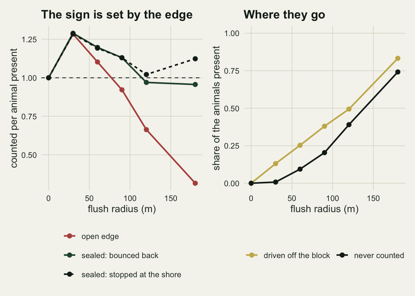
The survey herds what it does not lose
The lawnmower order is not symmetric. Each flush pushes an animal away from the aircraft, and the aircraft is always arriving from the strip it flew last, so the net push is in the direction the survey is advancing. In an open block that pushes animals over the far edge. In a sealed one it piles them up against it, and the per-strip count profile shows it directly.
flush_120 <- r120$flushes
flush_180 <- r180$flushes
lf_seal <- c(r30$last_first, r60$last_first, r120$last_first, r180$last_first)
strip_df <- do.call(rbind, lapply(c(0, 30, 60, 120), function(rf) {
  cc <- refl_cells[[which(rf_grid == rf)]]
  data.frame(strip = seq_along(cc$strip), count = cc$strip,
             r_f = factor(sprintf("%d m", rf), levels = sprintf("%d m", c(0, 30, 60, 120))))
}))
strip_open <- do.call(rbind, lapply(c(0, 30, 60, 120), function(rf) {
  cc <- open_cells[[which(rf_grid == rf)]]
  data.frame(strip = seq_along(cc$strip), count = cc$strip,
             r_f = factor(sprintf("%d m", rf), levels = sprintf("%d m", c(0, 30, 60, 120))))
}))
lf_zero <- refl_tab$last_first[refl_tab$r_f == 0]
move_120 <- r120$moving
move_180 <- r180$moving
disc_m <- 2 * max(rf_grid)
disc_strips <- disc_m / strip_m
disc_block <- disc_m / block_m
Inside the sealed block, with the animals bouncing back off the shore, each animal is flushed 3.4 times on average at a flush radius of 120 m and 6.6 times at 180 m. The last strip then records 1.4 times as many crossings as the first at 30 m, 2.1 at 60 m, 2.9 at 120 m and 5.2 at 180 m, against 0.96 when nothing flushes at all, which is the sampling noise in scattering three hundred animals over ten strips. A per-strip density gradient of that size in a real dataset would be read as habitat: better nesting substrate at one end of the colony, or a disturbance source at the other. It is the flight plan.
strip_col <- c("0 m" = te_body, "30 m" = te_forest, "60 m" = te_gold,
               "120 m" = te_rust)
p_seal <- ggplot(strip_df, aes(strip, count, colour = r_f)) +
  geom_line(linewidth = 0.9) +
  geom_point(size = 1.8) +
  scale_colour_manual(values = strip_col, name = "flush radius") +
  scale_x_continuous(breaks = 1:10) +
  labs(x = "strip, in flight order", y = "mean crossings recorded",
       title = "Sealed edge, bounced back") +
  theme_datasheet()
p_open <- ggplot(strip_open, aes(strip, count, colour = r_f)) +
  geom_line(linewidth = 0.9) +
  geom_point(size = 1.8) +
  scale_colour_manual(values = strip_col, name = "flush radius") +
  scale_x_continuous(breaks = 1:10) +
  labs(x = "strip, in flight order", y = "mean crossings recorded",
       title = "Open edge") +
  theme_datasheet()
p_seal + p_open + plot_layout(guides = "collect") +
  plot_annotation(theme = theme_datasheet()) &
  theme(legend.position = "bottom")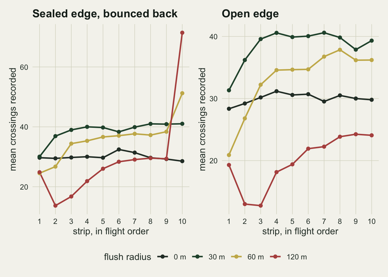
What carries the recount
The inflation side needs lateral flight. An animal that runs along the flight line, ahead of or behind the aircraft, stays in the strip it was already counted in and gets crossed again only if the drone overtakes it, which under the crossing rule it does once and no more. An animal that runs across the flight lines can land in ground the aircraft has not reached, and then be crossed a second time in the next strip.
set.seed(51105)
along_cells <- lapply(c(30, 60, 120), function(rf)
  run_cell(n_rep_side, r_f = rf, along_only = TRUE, head_sd = 0))
along_tab <- do.call(rbind, Map(function(rf, cc)
  data.frame(r_f = rf, ratio = cc$mean[["ratio"]], twice = cc$mean[["twice"]],
             never = cc$mean[["never"]], out = cc$mean[["out"]]),
  c(30, 60, 120), along_cells))
set.seed(51106)
refuge_cells <- list(
  `along the lines` = run_cell(n_rep_side, r_f = 60, refuge = 0),
  `across the lines` = run_cell(n_rep_side, r_f = 60, refuge = pi / 2))
refuge_tab <- do.call(rbind, lapply(names(refuge_cells), function(nm) {
  cc <- refuge_cells[[nm]]
  data.frame(arm = nm, ratio = cc$mean[["ratio"]], se = cc$se[["ratio"]],
             twice = cc$mean[["twice"]], never = cc$mean[["never"]],
             out = cc$mean[["out"]])
}))
ref_along  <- refuge_tab[refuge_tab$arm == "along the lines", ]
ref_across <- refuge_tab[refuge_tab$arm == "across the lines", ]
along_twice_max <- max(along_tab$twice)
Forcing every flush to run parallel to the flight lines removes the recount entirely. The share of animals counted twice or more is 0.000 at every flush radius tested, and the count comes to 0.989 at 30 m, 0.970 at 60 m and 0.947 at 120 m: below one at every radius, and below one only because animals still walk off the ends of the block.
Running away from the aircraft is one flight rule among several. A more realistic one for many species is running to cover, a fixed compass direction set by the terrain rather than by the drone. That version does not remove the problem; it makes the answer depend on how the flight plan happens to be oriented. With every animal at a flush radius of 60 m running along the flight lines, the count is 1.07. With every animal running across them, in the direction the survey advances, it is 2.60, with 0.68 of the animals counted twice or more and 0.70 driven off the far edge. An animal that keeps pace with the advancing survey gets photographed strip after strip.
carr_df <- data.frame(
  rule = c("away from the drone", "along the lines only",
           "refuge along the lines", "refuge across the lines"),
  ratio = c(o60$ratio, along_tab$ratio[2], ref_along$ratio, ref_across$ratio),
  twice = c(o60$twice, along_tab$twice[2], ref_along$twice, ref_across$twice))
carr_df$rule <- factor(carr_df$rule, levels = rev(carr_df$rule))
p_c1 <- ggplot(carr_df, aes(ratio, rule)) +
  geom_vline(xintercept = 1, linetype = "dashed", colour = te_body,
             linewidth = 0.5) +
  geom_segment(aes(x = 1, xend = ratio, y = rule, yend = rule),
               colour = te_line, linewidth = 1.2) +
  geom_point(size = 3.2, colour = te_forest) +
  labs(x = "counted per animal present", y = NULL,
       title = "Where the flush points") +
  theme_datasheet()
p_c2 <- ggplot(carr_df, aes(twice, rule)) +
  geom_segment(aes(x = 0, xend = twice, y = rule, yend = rule),
               colour = te_line, linewidth = 1.2) +
  geom_point(size = 3.2, colour = te_rust) +
  scale_x_continuous(limits = c(0, 0.8)) +
  labs(x = "share counted twice or more", y = NULL,
       title = "The recount follows it") +
  theme_datasheet() +
  theme(axis.text.y = element_blank())
p_c1 + p_c2 + plot_annotation(theme = theme_datasheet())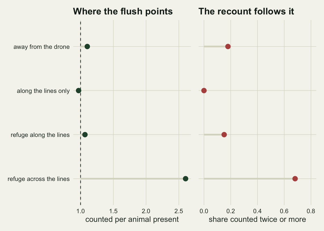
set.seed(51107)
half_cells <- lapply(c(30, 60, 120), function(rf)
  run_cell(n_rep_side, r_f = rf, pf = 0.5))
wide_cells <- lapply(c(30, 60, 120), function(rf)
  run_cell(n_rep_side, r_f = rf, head_sd = pi / 3))
dist_cells <- lapply(c(50, 150), function(df_m)
  run_cell(n_rep_side, r_f = 60, d_f = df_m))
grab <- function(cells) vapply(cells, function(cc) cc$mean[["ratio"]], 0)
half_ratio <- grab(half_cells)
wide_ratio <- grab(wide_cells)
dist_ratio <- grab(dist_cells)
side_se <- max(vapply(c(half_cells, wide_cells, dist_cells),
                      function(cc) cc$se[["ratio"]], 0))
Neither half of the pattern is an artefact of the two least defensible assumptions. Halving the response probability, so that only half the animals within the flush radius lift, gives 1.28, 1.15 and 0.66 at 30, 60 and 120 m against 1.28, 1.10 and 0.66 at full response. The one cell that moves is 60 m, where halving the probability raises the count rather than lowering it: fewer flushes means less emigration, so less of the recount is offset. Doubling the heading error to 60 degrees gives 1.29, 1.18 and 0.71. These side arms used 25 surveys per cell, with a Monte Carlo standard error of at most 0.009. The flush distance moves the result more than either: at a flush radius of 60 m, a 50 m flight gives 0.98 and a 150 m flight gives 1.17. It is the distance flown, not the probability of flying, that decides how far across the strip boundary the animal lands.
A wider flown area does not fix the count
The obvious repair for the deficit is to stop treating the block edge as the edge of the imaged area, so that animals pushed out of the core are still over ground the camera covers. The arm below is the simplest version of that: it enlarges the lawnmower. The core stays 800 m square and the population stays the 300 animals inside it at take-off, and the flown area is extended by 40, 80 or 160 m on all four sides, which adds one, two or four strips flown in the same back-and-forth order. That is not a perimeter lap flown before the core, which is a different design and is not simulated here: a perimeter lap sweeps the boundary while the core is still undisturbed, and pushes edge animals inward rather than outward. What is measured here is only whether flying a wider area repairs the count.
buf_grid <- c(0, 40, 80, 160)
set.seed(51108)
buf_tab <- do.call(rbind, lapply(c(60, 120), function(rf) {
  do.call(rbind, lapply(buf_grid, function(b) {
    cc <- run_cell(n_rep_buf, r_f = rf, buf = b)
    data.frame(r_f = sprintf("flush radius %d m", rf), buf = b,
               ratio = cc$mean[["ratio"]], se = cc$se[["ratio"]],
               never = cc$mean[["never"]], out = cc$mean[["out"]])
  }))
}))
b60  <- buf_tab[buf_tab$r_f == "flush radius 60 m", ]
b120 <- buf_tab[buf_tab$r_f == "flush radius 120 m", ]
b60_gain  <- b60$ratio[4] - b60$ratio[1]
b120_gain <- b120$ratio[4] - b120$ratio[1]
b120_short <- 1 - b120$ratio[4]
buf_se_max <- max(buf_tab$se)
At a flush radius of 60 m the buffer takes the count from 1.09 with no buffer to 1.16, 1.19 and 1.21 at 40, 80 and 160 m. The buffer worked, in the sense that the share of animals lost outside the flown area falls from 0.25 to 0.025. What it produced is not an unbiased count but a bias 0.12 higher, because removing the emigration removed the only thing that was offsetting the recount.
At 120 m the buffer does less than the arithmetic of the widths suggests. The count goes from 0.65 to 0.84, a gain of 0.19 that still leaves it 0.16 short of one, with 0.24 of the animals never crossed at all even though only 0.11 finished outside the flown area. A buffer of 160 m, wider than the 100 m the animals fly, does not return them, because an animal flushed repeatedly keeps moving ahead of the aircraft rather than being displaced once and settling. The buffer width that would be needed is not set by the flush radius or the flush distance but by their product with the number of flushes, and that number grows with the flown area. These cells used 20 surveys each, with a Monte Carlo standard error of at most 0.009. The contrast between no buffer and the widest one is many times that, but the three non-zero widths are two or three standard errors apart, so nothing here rests on their ordering.
buf_tab$r_f <- factor(buf_tab$r_f, levels = c("flush radius 60 m",
                                              "flush radius 120 m"))
ggplot(buf_tab, aes(buf, ratio, colour = r_f)) +
  geom_hline(yintercept = 1, linetype = "dashed", colour = te_body,
             linewidth = 0.5) +
  geom_line(linewidth = 0.9) +
  geom_point(size = 2.4) +
  scale_colour_manual(values = c("flush radius 60 m" = te_rust,
                                 "flush radius 120 m" = te_forest),
                      name = NULL) +
  labs(x = "buffer flown around the core (m)",
       y = "counted per animal present",
       title = "A buffer removes the loss, not the bias",
       subtitle = "core held at 800 m square; the count is per animal inside it at take-off") +
  theme_datasheet() +
  theme(legend.position = "bottom")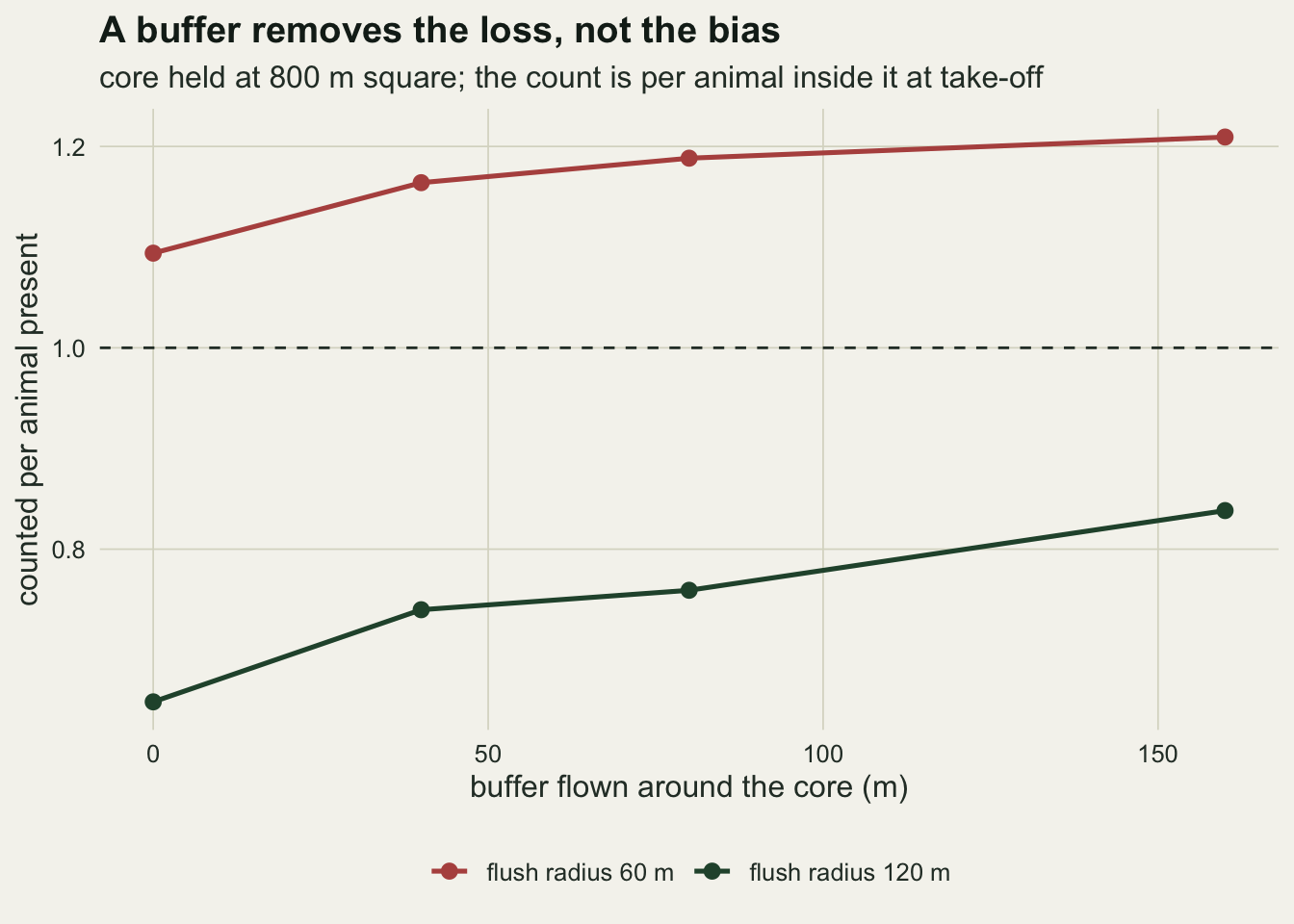
What to report
Report the flush radius, not the disturbance. Welfare reporting for drone work already asks for flight initiation distances, and those are the same numbers the count bias depends on. A survey that states a mean flight initiation distance of 30 m has said that its mosaic count is biased upward by something like 28 per cent before any detection or identification error is considered; a survey that states 120 m has said something much worse, and in the other direction.
Say whether the block has an edge the animals can leave through. This is the single piece of information that decides the sign. A colony on an island, a haulout ringed by water, a waterbird roost on an isolated lagoon: in all of these the sealed arm applies, the count is inflated, and at the flush radii of 30 to 60 m that a low multirotor provokes the inflation is between 1.19 and 1.29 per animal, whichever of the two shore rules is assumed. An open block of grassland or saltmarsh has the other problem. Do not carry the sealed result to a species that lifts at 120 m or more: there the two shore rules disagree, and the post reports no sealed number.
Give the per-strip count in flight order. It costs nothing, since the strip is already in the image metadata, and a gradient along the flight order is diagnostic. At a flush radius of 60 m in a sealed block the last strip held 2.1 times the crossings of the first, and no habitat gradient was simulated.
Do not report a wider flown area as a correction. Enlarging the block reduces the loss and raises the count, and at a flush radius of 60 m it raised it past one, from 1.09 to 1.21. A buffer is a way to stop the emigration, which makes the remaining bias one-signed and therefore easier to reason about, but it is not a correction factor and should not be quoted as one.
Honest limits
The counting rule here is exact, which is not a modest assumption. There is no detection probability, no missed animal under vegetation, no false positive on a rock, and no identification error at all. Real image counts have all four, and the identification side is what the deduplication literature is about. The point of removing them is to show that a count bias of this size survives their absence, not to suggest that they are small.
The flight response is a hard radius with a fixed flight distance. Real flight initiation distances have a distribution, they depend on approach geometry and altitude, they habituate within a survey and between surveys, and an animal that has just been flushed is more likely to flush again, not equally likely. The response probability arm shows the pattern surviving a halved probability, and the heading arm shows it surviving a doubled heading error, but neither of those is a model of habituation, and a strong habituation would cut the repeated-flush deficit specifically.
The animals do not interact. A colony flushes in sheets, not one bird at a time, and a correlated flush moves a block of animals together, which would change the double-count share and the per-strip profile in ways that independent flushing cannot show. The same applies to the sealed edge: it is an idealisation of water or a fence, not of a habitat boundary that animals are reluctant but able to cross.
The block is flown once, in one direction, with no overlap between strips. Practitioners fly with sidelap, and the twice-imaged seam between adjacent strips is exactly where a displaced animal is most likely to be seen twice by a matching rule and reconciled. A sidelap design would reduce the recount measured here to the extent that the matching works, and would leave the emigration side untouched.
The 800 m block is small, and the deficit scales with perimeter over area. The same flush radius on a 3 km block loses a smaller share of the population and would show a milder undercount, because fewer animals start within reach of an edge. Nothing here should be read as a bias for drone surveys in general: the numbers belong to this block size, this strip width, this speed and these flight rules, and the transferable part is the mechanism and the sign.
The sealed edge is run under two rules because the easiest rule to write is not a neutral one. Mirroring a flushed animal’s position back across the boundary and leaving its heading alone pins a bird that is still in flight against the wall, step after step, until its flight distance runs out: that is a coding convention and not a behaviour, and it is the version this post does not use. Reversing the outward component of the heading, which is the textbook reflecting boundary, and ending the flight at the shore are the two defensible readings, and they are the two reported. Up to 90 m they agree to within 0.005 per animal, closer than the rounding in the list above suggests. Beyond 100 m they disagree by as much as 0.17, which is more than the largest departure from one that either of them shows there (0.12), and they disagree in sign: at 120 m the bouncing rule gives 0.97 and the stopping rule 1.02. Nothing about the sign of the sealed bias can be concluded in that range, and the post concludes nothing there.
The stopping rule also puts a strain on the counting rule that is worth naming. An animal that ends its flight at the shore rests exactly on the block boundary, and the outermost strip is the one whose centre lies half a strip width inside it, so the lateral test has to treat the shore line as part of that strip. The code settles the animal a hair inside the boundary for this reason. Left exactly on the line, with a strict inequality in the test, animals at the higher flush radii would sit where no strip can reach them, and the stopping rule would report an undercount that is a property of the arithmetic rather than of the survey.
The large radii are a different regime in any case. At a flush radius of 180 m the flush disc is 360 m across, which is 4.5 strip widths and 0.45 of the block in each direction, so the aircraft is provoking animals in strips it has not reached yet rather than in the strip it is flying. Each animal is then flushed 6.6 times and spends 0.27 of the flight in the air, against 0.14 at 120 m. Those cells are kept because the grid was fixed in advance, not because a real flight response is expected to look like that.
References
Turnock BJ, Quinn TJ 1991 Biometrics 47(2):701-715 (10.2307/2532156)
Buckland ST, Turnock BJ 1992 Biometrics 48(3):901-909 (10.2307/2532356)
Glennie R, Buckland ST, Thomas L 2015 PLoS ONE 10(3):e0121333 (10.1371/journal.pone.0121333)
Mulero-Pazmany M, Jenni-Eiermann S, Strebel N, Sattler T, Negro JJ, Tablado Z 2017 PLoS ONE 12(6):e0178448 (10.1371/journal.pone.0178448)
Hodgson JC, Koh LP 2016 Current Biology 26(10):R404-R405 (10.1016/j.cub.2016.04.001)
Brack IV, Kindel A, Oliveira LFB 2018 Methods in Ecology and Evolution 9(8):1864-1873 (10.1111/2041-210X.13026)