library(ggplot2)

te_paper  <- "#f5f4ee"
te_ink    <- "#16241d"
te_body   <- "#2c3a31"
te_forest <- "#275139"
te_rust   <- "#b5534e"
te_gold   <- "#c9b458"
te_line   <- "#dad9ca"

theme_datasheet <- function() {
  theme_minimal(base_size = 12) +
    theme(plot.background  = element_rect(fill = te_paper, colour = NA),
          panel.background = element_rect(fill = te_paper, colour = NA),
          panel.grid.major = element_line(colour = te_line, linewidth = 0.3),
          panel.grid.minor = element_blank(),
          text             = element_text(colour = te_body),
          plot.title       = element_text(colour = te_ink, face = "bold"),
          plot.subtitle    = element_text(colour = te_body),
          axis.text        = element_text(colour = te_body))
}Pitfall catches and the depletion zone
R
pitfall traps
sampling
movement ecology
simulation
ecology tutorial
A pitfall keeps what it catches, so nearby beetles thin out. Simulating in R how that depletion zone bends the effort offset and how diffusion sets its size.
A line of pitfall traps along a woodland edge, plastic cups sunk flush with the soil, emptied once a week. Some lines stay out for a week because the site is a long drive away; others stay out for four weeks because the landowner is relaxed about it. The catches are ground beetles, and the analysis divides them by trap-days, or does the same thing properly with a log offset in a Poisson model.
The post on offsets for rates and densities builds exactly this kind of synthetic pitfall study and states the assumption behind the offset plainly: the expected count is density multiplied by effort, so the log of effort enters with a coefficient of exactly one. In that post the counts are generated to obey it, which is the right way to teach an offset. The question here is whether a pitfall can obey it at all. A pitfall is not a window onto a fixed rate. It is a hole that keeps what falls in, and every beetle it keeps is one fewer beetle walking near the hole.
That sounds like the removal model, and the post on removal and depletion sampling covers the classical version: a closed patch, several passes, each animal caught with the same probability on every pass. There is no space in that model; the whole population is equally exposed to the gear. A pitfall is the opposite case. It is tiny, the population around it is effectively unbounded, and only the beetles that happen to be close are at risk. Removal can only thin the ground near the cup, and how far that thinning reaches depends on how the beetles move.
Movement is also where the third neighbour comes in. The post on the random encounter model for camera traps derives an encounter rate proportional to density times speed, for a detector that removes nothing (the ideal gas model that Hutchinson and Waser 2007 review across animal encounter problems). A pitfall is that detector with removal switched on. Greenslade 1964 and Topping and Sunderland 1992 made the field version of the point long ago: pitfall catches measure activity as much as abundance. Part of that point needs no simulation: a trap that removed nothing would catch in proportion to speed, straight from the encounter formula. What the formula cannot give is how much of that catch a trap that keeps its beetles actually makes, how deep the thinned zone around it is, and how far the catch per day drifts as a session lengthens. Those are the things this post measures, with nothing but random walks and a disc.
A walk with a hole in the ground
trap_r   <- 0.05                   # pitfall radius in metres (a 10 cm cup)
dt_h     <- 1                      # hours between changes of direction
n_days   <- 28                     # session length
n_step   <- n_days * 24 / dt_h     # steps in a session
dens     <- 1                      # beetles per square metre, everywhere and always
step_grid <- c(0.25, 0.5, 1, 2)    # metres walked in one hour
diff_D    <- step_grid^2 / (4 * dt_h)                   # square metres per hour
width_grid <- pmax(20, 2 * sqrt(4 * diff_D * n_step))   # side of the torus, metres
ceiling_28 <- 2 * trap_r * step_grid * dens * n_step    # no-depletion catch per trap
n_trap_grid <- ceiling(5000 / ceiling_28)               # traps simulated per step length

# every trap sits at the centre of its own torus; animals are independent,
# so all tori are walked together in one set of vectors
walk_traps <- function(step_len, n_trap, width, remove = TRUE, snap = integer(0), n_ring = 10,
                       n_steps = n_step) {
  n_per   <- rpois(n_trap, dens * width^2)
  trap_id <- rep(seq_len(n_trap), n_per)
  half <- width / 2
  px <- runif(length(trap_id), -half, half); py <- runif(length(trap_id), -half, half)
  outside <- px^2 + py^2 > trap_r^2
  px <- px[outside]; py <- py[outside]; trap_id <- trap_id[outside]
  n_anim <- length(px)
  cap_step <- integer(0); cap_trap <- integer(0)
  reach2 <- (step_len + trap_r)^2
  ring_brk <- c(trap_r, 0.25 * (half / 0.25)^seq(0, 1, length.out = n_ring + 1)); rings <- list()
  for (s in seq_len(n_steps)) {
    ang <- runif(n_anim, 0, 2 * pi)
    dx <- step_len * cos(ang); dy <- step_len * sin(ang)
    near <- which(px * px + py * py < reach2)
    if (length(near)) {
      qx <- px[near]; qy <- py[near]; ex <- dx[near]; ey <- dy[near]
      u <- pmin(1, pmax(0, -(qx * ex + qy * ey) / step_len^2))   # closest point on the step
      hit <- near[(qx + u * ex)^2 + (qy + u * ey)^2 < trap_r^2 & qx^2 + qy^2 >= trap_r^2]
      if (length(hit)) {
        cap_step <- c(cap_step, rep(s, length(hit))); cap_trap <- c(cap_trap, trap_id[hit])
        if (remove) {        # the captured beetle is replaced by one dropped anywhere on the torus
          px[hit] <- runif(length(hit), -half, half); py[hit] <- runif(length(hit), -half, half)
          dx[hit] <- 0; dy[hit] <- 0
        }
      }
    }
    px <- px + dx; py <- py + dy
    if (s %% 8 == 0 || s %in% snap) {
      px <- (px + half) %% width - half; py <- (py + half) %% width - half
    }
    if (s %in% snap) {
      rr <- sqrt(px^2 + py^2)
      rings[[as.character(s)]] <- tabulate(findInterval(rr[rr < half], ring_brk), length(ring_brk) - 1)
    }
  }
  list(cap_step = cap_step, cap_trap = cap_trap, n_anim = n_anim, n_trap = n_trap,
       width = width, step_len = step_len, rings = rings, ring_brk = ring_brk)
}
The model is deliberately plain. Beetles walk in straight segments and pick a new, uniformly random direction every hour. The cup is a disc of radius 0.05 m, and a beetle is caught if its path during an hour passes over the disc, so a fast walker cannot step over the trap between two positions. Density is 1 beetle per square metre, and the step lengths are 0.25, 0.50, 1.00, 2.00 metres per hour. All of these are design constants fixed before any run.
Two clocks matter. At the scale of the cup the walk is a straight line, and what counts is the speed, the step length per hour. At the scale of metres and days the walk is diffusion, with a diffusion coefficient of step length squared over four times the time step: 0.375, 1.5, 6, 24 square metres per day for the four step lengths.
Each trap sits in the middle of a square torus, so there are no edges. The side of the torus is twice the diffusion distance over the whole session (with a floor of 20 m), which gives 20, 26, 52, 104 m. One more rule keeps global depletion out of the picture entirely: a captured beetle is replaced by a new one dropped at a uniformly random point on the torus. The density of the torus as a whole never changes, so anything that falls over the session is a local effect. Because the beetles never interact, many traps can be walked in one set of vectors, each beetle labelled with its own torus.
set.seed(611)
n_walker <- 4000
end_x <- rowSums(matrix(cos(runif(n_walker * n_step, 0, 2 * pi)), n_walker))
end_y <- rowSums(matrix(sin(runif(n_walker * n_step, 0, 2 * pi)), n_walker))
msd_ratio <- mean(end_x^2 + end_y^2) / (4 * (1^2 / (4 * dt_h)) * n_step)
msd_se <- sd(end_x^2 + end_y^2) / sqrt(n_walker) / (4 * (1^2 / (4 * dt_h)) * n_step)
A quick check that the diffusion coefficient means what it says: 4000 free walkers with a one metre step, no trap, one session. Their mean squared displacement is 1.016 times the diffusion prediction of four times the coefficient times the time, with a Monte Carlo standard error of 0.016. That is just the sum of independent steps, but it confirms the scaling used in every number below.
A trap that does not keep what it catches
set.seed(612)
ctr <- walk_traps(step_len = 1, n_trap = 30, width = 20, remove = FALSE)
ctr_expect <- 2 * trap_r * 1 * dens * n_step * ctr$n_anim / (30 * 20^2)
ctr_obs <- length(ctr$cap_step) / 30
ctr_se <- sqrt(length(ctr$cap_step)) / 30
ctr_half <- c(sum(ctr$cap_step <= n_step / 2), sum(ctr$cap_step > n_step / 2))
Before any removal, a control. Here the trap counts every beetle whose path enters the disc but lets it walk on. The encounter-rate argument from the camera trap post gives the expected count directly: a disc has perimeter two pi times its radius, and the rate is density times speed times perimeter over pi, which is twice the radius times the step length per hour. Over 672 hours on 30 tori that predicts 67.2 beetles per trap (at the realised density of the draws). The simulation gives 68.8, with a Poisson standard error of 1.5. The first half of the session produces 1022 entries and the second half 1042, so a trap that keeps nothing keeps a constant rate.
Call this the no-depletion ceiling: the catch a trap would make if nothing were ever removed. It already contains one result that looks like a finding. At equal density the ceiling is proportional to step length per hour, so doubling the speed doubles it, and going from a quarter of a metre to two metres multiplies it by 8. Nothing below needs a simulation to say that. What the simulation adds is the fraction of the ceiling a trap that keeps its catch actually retains.
The zone
set.seed(2828)
t_main <- system.time(
  sims <- lapply(seq_along(step_grid), function(k)
    walk_traps(step_grid[k], n_trap_grid[k], width_grid[k],
               snap = c(4:7, 25:28) * 24))
)[["elapsed"]]

week_days <- c(7, 14, 21, 28)
cum_mat <- function(sim) {
  daily <- tabulate((sim$cap_trap - 1) * n_days + ceiling(sim$cap_step * dt_h / 24),
                    sim$n_trap * n_days)
  daily <- matrix(daily, nrow = sim$n_trap, byrow = TRUE)
  t(apply(daily, 1, cumsum))[, week_days, drop = FALSE]
}
cums <- lapply(sims, cum_mat)
pois_slope <- function(tot) {
  unname(glm.fit(cbind(1, log(week_days)), tot, family = poisson())$coefficients[2])
}
set.seed(2829)
n_boot <- 400
summ <- do.call(rbind, lapply(seq_along(sims), function(k) {
  cm <- cums[[k]]; tot <- colSums(cm); wk <- diff(c(0, tot))
  boot <- replicate(n_boot, {
    bt <- colSums(cm[sample(nrow(cm), replace = TRUE), , drop = FALSE])
    c(pois_slope(bt), diff(c(0, bt))[4] / bt[1])
  })
  data.frame(step = step_grid[k], D_day = 24 * diff_D[k], width = width_grid[k],
             n_trap = n_trap_grid[k], catch = tot[4], per_trap = tot[4] / n_trap_grid[k],
             slope = pois_slope(tot), slope_se = sd(boot[1, ]),
             w41 = wk[4] / wk[1], w41_se = sd(boot[2, ]),
             closed_loss = tot[4] / sims[[k]]$n_anim,
             retained = tot[4] / n_trap_grid[k] / ceiling_28[k])
}))
bias_7_28 <- 4^(summ$slope - 1)     # 28-day rate per day relative to the 7-day rate
The number of traps for each step length was set before running, to give an expected catch of around five thousand under the ceiling: 298, 149, 75, 38 traps. Every trap runs the full 28 days, and the cumulative catch is read off at the end of each week. The effort exponent is the coefficient of log(days) in a Poisson regression of pooled cumulative catch on log(days); its standard error comes from 400 bootstrap resamples of traps, because the four cumulative totals from one trap are nested and a model-based standard error would treat them as independent.
The replacement rule was not idle. Without it, the tori would have lost 2.4, 3.6, 2.1, 1.1 per cent of their beetles over the session, which would lower the density the trap samples by up to that fraction by week four and would be mixed into the local effect with no way to separate the two.
prof <- do.call(rbind, lapply(sims, function(sim) {
  brk <- sim$ring_brk; area <- pi * (brk[-1]^2 - brk[-length(brk)]^2)
  snap_day <- as.integer(names(sim$rings)) / 24
  cnt_w1 <- Reduce(`+`, sim$rings[snap_day <= 7]); cnt_w4 <- Reduce(`+`, sim$rings[snap_day >= 25])
  dens_w1 <- cnt_w1 / (4 * sim$n_trap * area); dens_w4 <- cnt_w4 / (4 * sim$n_trap * area)
  far_rings <- length(area) - 1:0      # the two outermost rings stand for the far field
  data.frame(step = sim$step_len, time = factor(rep(c("days 4 to 7", "days 25 to 28"), each = length(area)), levels = c("days 4 to 7", "days 25 to 28")),
             dist = rep(c(0.15, sqrt(brk[-(1:2)] * brk[-c(1, length(brk))])), 2),
             rel = c(dens_w1 / mean(dens_w1[far_rings]), dens_w4 / mean(dens_w4[far_rings])),
             half_width = sim$width / 2)
}))
prof$panel <- factor(sprintf("%.2f m per hour", prof$step), levels = sprintf("%.2f m per hour", step_grid))
near_rel <- sapply(step_grid, function(s) prof$rel[prof$step == s & prof$time == "days 25 to 28"][1])ggplot(prof, aes(dist, rel, colour = time)) +
geom_hline(yintercept = 1, linetype = "dashed", colour = te_body) +
geom_line(linewidth = 0.7) + geom_point(size = 1.3) +
facet_wrap(~ panel) +
scale_x_log10(breaks = c(0.3, 1, 3, 10, 30), labels = c("0.3", "1", "3", "10", "30")) +
scale_colour_manual(values = c(te_gold, te_rust), name = NULL) +
labs(x = "distance from the pitfall centre (m, log scale)", y = "beetle density relative to far field") +
theme_datasheet() +
theme(legend.position = "bottom", strip.text = element_text(colour = te_ink, face = "bold"))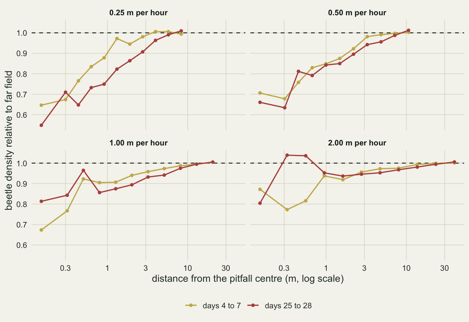
The zone is there for every step length, and it is shaped by movement. In the innermost ring, from the cup edge out to a quarter of a metre, the density over the last four days is 0.55 of the far field for the slowest walkers and 0.66 for the next. For the two faster step lengths the inner rings hold few beetles in the simulation and the line jumps around; the rings from one metre outwards are the ones to read, and there the deficit is shallower and reaches further out. Slow walkers dig a deep, narrow hole in the population; fast walkers a shallow, wide one. The slow profile also moves outwards between the first and fourth week, which is the zone growing.
Catch per day falls, slowly
ggplot(summ, aes(step, slope)) +
  geom_hline(yintercept = 1, linetype = "dashed", colour = te_body) +
  geom_errorbar(aes(ymin = slope - 2 * slope_se, ymax = slope + 2 * slope_se),
                width = 0.06, colour = te_forest) +
  geom_point(colour = te_forest, size = 2.8) +
  scale_x_log10(breaks = step_grid) +
  labs(x = "metres walked per hour (log scale)", y = "effort exponent on trap-days") +
  theme_datasheet()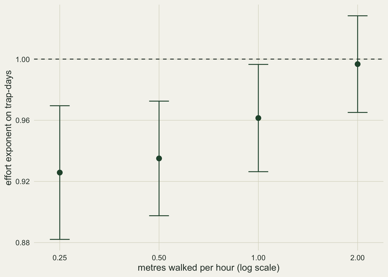
The exponents are 0.926, 0.935, 0.961, 0.997 for step lengths of 0.25, 0.50, 1.00, 2.00 m, with bootstrap standard errors of 0.016 to 0.022. The slowest walkers sit 3.4 standard errors below one; the fastest cannot be told from one. The same pattern shows in the weekly catches: week four divided by week one is 0.85, 0.87, 0.92, 0.96, each with a standard error near 0.04.
So the depletion zone bends the offset, but not by much. With a 10 cm cup, hourly turns and global depletion removed, the exponent stays above 0.92. The usual explanation is geometric: in two dimensions a small absorbing disc depletes its neighbourhood only logarithmically in time, because the beetles lost near the cup are refilled from an area that grows as fast as the zone does.
What the exponent means for an offset is modest. Compare a one-week and a four-week session at the same site. With an exponent of 0.926, the four-week catch per trap-day is 0.90 of the one-week rate for the slowest walkers, and 1.00 for the fastest. That is a real bias that depends on habitat, and it is small next to the next section.
Same density, different catch
speed_ratio <- summ$per_trap[-1] / summ$per_trap[-nrow(summ)]
end_ratio   <- summ$per_trap[4] / summ$per_trap[1]
d_ratio     <- diff_D[4] / diff_D[1]
ceil_ratio  <- step_grid[4] / step_grid[1]                    # from the formula alone
keep_ratio  <- summ$retained[4] / summ$retained[1]            # measured
per_trap_se <- function(sim, ceil) {
  sd(tabulate(sim$cap_trap, sim$n_trap)) / sqrt(sim$n_trap) / ceil
}
Hold density fixed at one beetle per square metre and change nothing but the step length.
ggplot(summ, aes(step, per_trap)) +
  geom_line(aes(y = 2 * trap_r * step * dens * n_step), linetype = "dashed", colour = te_body) +
  geom_line(colour = te_forest, linewidth = 0.8) +
  geom_point(colour = te_forest, size = 2.8) +
  annotate("text", x = 0.26, y = 62, label = "no-depletion ceiling (dashed)", colour = te_body, hjust = 0) +
  annotate("text", x = 1.1, y = 40, label = "simulated catch", colour = te_forest, hjust = 0) +
  scale_x_log10(breaks = step_grid) + scale_y_log10() +
  labs(x = "metres walked per hour (log scale)",
       y = "beetles per trap in 28 days (log scale)") +
  theme_datasheet()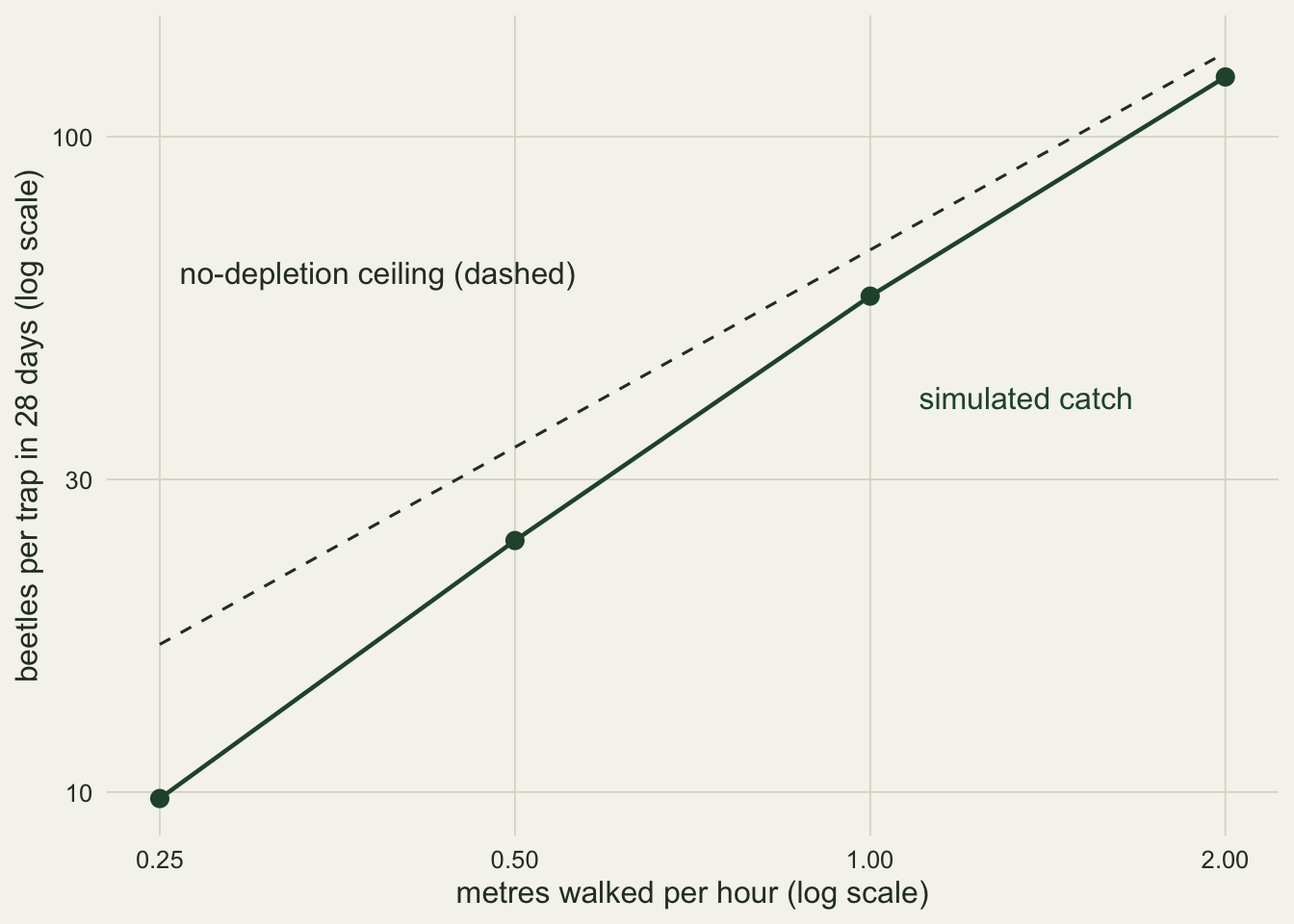
Catch per trap over the session is 9.8, 24.2, 57.1, 123.4 beetles for step lengths of 0.25, 0.50, 1.00, 2.00 m per hour. Each doubling of the step multiplies the catch by 2.48, 2.36, 2.16, and from the slowest to the fastest walkers the catch rises 12.6 times, at identical density.
Most of that is the ceiling. Two of each doubling ratio, and 8 of the 12.6, follow from the encounter formula alone. The simulation adds the rest: the slowest walkers deliver 58 per cent of their ceiling and the fastest 92 per cent, a factor of 1.58 on top of the 8. That factor is the depletion zone at work, and it is the only part of the range that a pitfall adds to what any detector of walking animals would show.
Speed or diffusion?
In the design above a longer step changes two things at once. With the turning time fixed at one hour, doubling the step doubles the speed and multiplies the diffusion coefficient by four. They can be pulled apart by changing the turning time as well, and running the same walk twice more.
set.seed(2830)
run_alt <- function(speed, dt_alt) {
  step_alt <- speed * dt_alt
  d_alt    <- step_alt^2 / (4 * dt_alt)
  width    <- max(20, 2 * sqrt(4 * d_alt * n_days * 24))
  ceil     <- 2 * trap_r * speed * dens * n_days * 24
  n_tr     <- ceiling(5000 / ceil)
  sim <- walk_traps(step_alt, n_tr, width, n_steps = round(n_days * 24 / dt_alt))
  data.frame(speed = speed, dt = dt_alt, D_day = 24 * d_alt, n_trap = n_tr,
             per_trap = length(sim$cap_step) / n_tr, retained = length(sim$cap_step) / n_tr / ceil,
             retained_se = per_trap_se(sim, ceil))
}
alt <- rbind(run_alt(0.5, 0.25),     # twice the speed, the diffusion of the slowest walkers
             run_alt(0.25, 4))       # the slowest speed, the diffusion of the half metre walkers
base_se <- per_trap_se(sims[[1]], ceiling_28[1])
fast_same_D  <- alt$per_trap[1] / summ$per_trap[1]
slow_more_D  <- alt$per_trap[2] / summ$per_trap[1]
The first extra run keeps the diffusion coefficient of the slowest walkers, 0.375 square metres per day, but doubles their speed to half a metre an hour by turning every 0.25 hours. The second keeps the slowest speed but turns only every 4 hours, which gives it the diffusion coefficient of the half metre walkers, 1.5 square metres per day. Tori and trap numbers follow the same rules as before (149 and 298 traps).
Against the slowest walkers of the main design, who catch 9.8 per trap and retain 0.58 of the ceiling (standard error 0.012), doubling speed at fixed diffusion gives 12.3 per trap, only 1.26 times as many. The ceiling doubled, but the retained fraction fell to 0.37 (standard error 0.009): faster walkers empty their own neighbourhood faster, and the neighbourhood refills no faster than before. Quadrupling diffusion at fixed speed leaves the ceiling where it was and gives 14.6 per trap, 1.50 times as many, because the retained fraction rises to 0.87 (standard error 0.013).
So the part of the speed effect that the formula does not give comes from diffusion, not from speed: at fixed diffusion extra speed lowers the retained fraction, and only the fourfold rise in diffusion that comes with each doubled step raises it. Diffusion here is set by a turning time of one hour that was chosen for convenience, not measured on any beetle. The 1.58 above is tied to that choice: longer turning times push the retained fraction towards one, as the second run shows, and leave less room for it. What does not depend on the turning time is the direction: walkers that cover more ground between turns keep their trap closer to its ceiling, and a pitfall catch cannot tell that apart from density. An effort offset cannot touch it either, because the effort is the same.
What a field study sees
set.seed(4417)
n_site <- 60
pick_sites <- function(k, habitat) {
  rows <- sample(nrow(cums[[k]]), n_site)
  week_col <- sample(4, n_site, replace = TRUE)
  data.frame(habitat = habitat, days = week_days[week_col], count = cums[[k]][cbind(rows, week_col)])
}
study <- rbind(pick_sites(2, "litter"), pick_sites(3, "open"))
study$habitat <- factor(study$habitat, levels = c("litter", "open"))
m_off  <- glm(count ~ habitat + offset(log(days)), family = poisson, data = study)
m_free <- glm(count ~ habitat + log(days), family = poisson, data = study)
ratio_off <- exp(coef(m_off)[["habitatopen"]])
ratio_ci  <- exp(confint.default(m_off)["habitatopen", ])
b_free    <- coef(m_free)[["log(days)"]]
b_ci      <- confint.default(m_free)["log(days)", ]
disp_off  <- sum(residuals(m_off, type = "pearson")^2) / df.residual(m_off)
Put the two effects in front of a model. Take 60 traps from the half metre walkers, call them leaf litter, and 60 from the one metre walkers, call them open ground; give each trap a session of one to four weeks at random. Density is identical in both habitats by construction.
The offset model, the one recommended for exactly this kind of data, estimates that open ground holds 2.28 times the beetles of leaf litter, with a Wald interval from 2.11 to 2.46. Nothing in the fit warns about this: the Pearson dispersion is 0.88. Freeing the coefficient on log(days) instead of fixing it gives 0.939, with an interval from 0.855 to 1.023, which includes one. A study of this size cannot see the depletion zone in its effort exponent, and it is fooled by movement in its habitat comparison. Two of the 2.28 is the speed ratio itself, which the encounter formula would predict for any detector; the remaining factor of 1.14 stands for the ratio of retained fractions between the two walkers, which is 1.18 in the full simulation.
What to report
Call a pitfall catch activity density, and mean it. The number is a product of density and movement: a 12.6-fold range from movement alone in the simulation above, of which 8 is plain speed and the rest is how much of its ceiling a trap keeps, which depends on how often the walkers turn. A comparison of habitats, seasons or treatments that change how beetles walk is a comparison of that product.
If session lengths differ, report them, and do not rely on the offset alone to make them comparable. For the slowest walkers here the four-week rate fell about 10 per cent below the one-week rate (from 4 to 15 per cent within two standard errors of the exponent), and the fall would be larger for walkers slower or more tortuous than these; nothing in a small data set reveals it. Equal session lengths remove the question.
When the question is density rather than activity, pitfalls need a second source of information about movement, just as the random encounter model needs speed from somewhere else: mark-release to estimate displacement, enclosures of known density to calibrate the catch, or a design that compares like with like in structure and temperature.
Honest limits
The walk is uncorrelated, with a fixed hourly turning time and no rest. Real carabids alternate bursts of directed walking with long stops, turn more in dense vegetation, and many have home ranges or retreat to shelter by day. A bounded or site-faithful walk refills the zone more slowly than the open diffusion used here, so the exponents above are likely the gentle end of what a pitfall does. The step length in the main design changed speed and diffusion together. The two extra runs separate them at one point of the grid only, and they show that the depletion part of the speed effect depends on a turning time that is a modelling choice; a study that wants the size of that part for a real species needs its turning behaviour.
The trap is a single cup. A grid of traps shares one depletion field, and traps a few metres apart compete for the slow walkers. On the torus each trap sees periodic copies of itself at the torus width, which is a very sparse grid; the far field density used for scaling is taken from the outer rings, which is only fair if the copies are far enough apart, and for the slowest walkers the profile is still rising at a few metres.
Everything else a pitfall does is absent. There is no digging-in effect (a change in catch in the days after installation), no escape from the cup, no weather-driven activity, no preservative that attracts or repels. Those act on the same weekly catch, and any of them can be as large as the depletion bias measured here.
The inner rings of the profile figure hold few simulated beetles for the fast walkers and should be read as noise. The exponent standard errors are bootstrap over traps, and the four exponents are separated by only a few of them; only the two ends of the range are clearly apart, and neighbouring step lengths are not. Finally, the one closed-form expression used, the no-depletion ceiling, was checked against the simulation and serves only as a reference; the depletion results come from the walks, not from a formula.
References
Greenslade PJM 1964 Journal of Animal Ecology 33(2):301 (10.2307/2632)
Topping CJ, Sunderland KD 1992 Journal of Applied Ecology 29(2):485-491 (10.2307/2404516)
Hutchinson JMC, Waser PM 2007 Biological Reviews 82(3):335-359 (10.1111/j.1469-185X.2007.00014.x)