library(ggplot2)
library(patchwork)

te_paper  <- "#f5f4ee"
te_ink    <- "#16241d"
te_body   <- "#2c3a31"
te_forest <- "#275139"
te_rust   <- "#b5534e"
te_gold   <- "#c9b458"
te_line   <- "#dad9ca"

theme_datasheet <- function() {
  theme_minimal(base_size = 12) +
    theme(plot.background  = element_rect(fill = te_paper, colour = NA),
          panel.background = element_rect(fill = te_paper, colour = NA),
          panel.grid.major = element_line(colour = te_line, linewidth = 0.3),
          panel.grid.minor = element_blank(),
          text             = element_text(colour = te_body),
          plot.title       = element_text(colour = te_ink, face = "bold"),
          plot.subtitle    = element_text(colour = te_body),
          axis.text        = element_text(colour = te_body),
          strip.text       = element_text(colour = te_ink))
}Flight-season shifts and false occupancy trends
R
occupancy
phenology
imperfect detection
citizen science
simulation
ecology tutorial
A flight season moving towards the edge of a fixed recording window gives a false occupancy decline that a year term on detection misses. Simulated in R.
A county butterfly recording scheme takes records of a small, short-lived species between 30 May and 18 August and has done so for ten years. Every year roughly the same number of recorders go out, each makes a handful of trips to a favourite site in a week or two that suits them, and the records go into an occupancy model with a trend on the occupancy scale. Over the same ten years the flight season has come forward by about three days a year. The trend comes out negative, and the question a referee will ask is whether the species is losing sites or whether it is simply flying before the recorders are out.
The general version of that question is already answered on this site. Open N-mixture models and the detection trap lets detection fall by year and shows that a constant-detection model turns a growing population into a shrinking one, while a model with logit detection linear in year, identified by the repeat visits within each spring, recovers the trend. Covariates in dynamic occupancy models leaves a real detection covariate out and watches its effect reappear in extinction. Both posts carry the same lesson: a change in detection that the model does not include ends up in the state process. The obvious reading for the butterfly is to put a year term on detection and move on.
This post is about the case where that reading fails. A moving flight season is a detection change that acts through the visit dates, not through the year, and what a year term on detection can absorb depends on two things the neighbour posts had no reason to vary: where the season sits in the recording window, and whether a site’s visits are spread through the season or bunched in one part of it. Occupancy from unstructured records names the related worry in its honest limit (a species that arrives or leaves mid-season was not measured there), and checking a phenology analysis shows the survey window cutting off the start of a season when the quantity of interest is a date. Here the quantity of interest is occupancy and the season is inside the window for most of its length.
None of the ingredients is new. Seasonal detectability curves inside occupancy models were used by Strebel and colleagues in 2014 to read the date of peak detectability as a phenological measure, Roth, Strebel and Amrhein adapted site-occupancy models to estimate phenological trends in the same year, and van Strien, van Swaay and Termaat showed that occupancy models fitted to opportunistic records of butterflies and dragonflies give usable distribution trends. That detection heterogeneity among sites biases occupancy downwards is the subject of Royle’s 2006 paper. What the post measures is the size of the false trend each of five fitting choices produces when a season moves, with the position of the season in the window as a required axis of the design.
A recording window that stays put
The simulation keeps everything fixed except the season. There are 300 sites and ten years, and each site-year is treated as its own closed occupancy unit with true occupancy 0.4 in every year, so the true trend is zero. Detection on a visit is a Gaussian curve in day of year with a height of 0.6 and a standard deviation of 12 days; its peak moves 3 days earlier each year. Recording is accepted only between day 150 and day 230, and every site-year gets four visits.
The peak position is the axis the whole post turns on, so it has two levels fixed before any fitting ran. In the central geometry the middle-year peak sits at day 190, the centre of the window, and the ten peaks run symmetrically either side of it. In the edge geometry the middle-year peak is day 172, so the season starts in the middle of the window and runs towards the opening date. Visit days are either independent and uniform across the window, or bunched: each site-year draws a centre date uniformly in the window and its visits scatter normally around that centre with a standard deviation of 5 or 14 days, a visit that falls outside the window being moved to the nearest window edge.
n_site    <- 300
n_year    <- 10
psi_true  <- 0.4
p_max     <- 0.6
season_sd <- 12
win_lo    <- 150
win_hi    <- 230
shift_use <- -3
mid_central <- 190
mid_edge    <- 172
n_visit_use <- 4

year_c   <- seq_len(n_year) - (n_year + 1) / 2
unit_yc  <- rep(year_c, each = n_site)
unit_yr  <- rep(seq_len(n_year), each = n_site)

sim_records <- function(peak_mid, shift, clus_sd, n_visit, trend = 0) {
  n_unit <- n_site * n_year
  z_unit <- rbinom(n_unit, 1, plogis(qlogis(psi_true) + trend * unit_yc))
  if (clus_sd == 0) {
    days <- matrix(runif(n_unit * n_visit, win_lo, win_hi), n_unit)
  } else {
    centre <- runif(n_unit, win_lo, win_hi)
    days <- centre + matrix(rnorm(n_unit * n_visit, 0, clus_sd), n_unit)
    days <- pmin(pmax(days, win_lo), win_hi)
  }
  peak  <- peak_mid + shift * unit_yc
  p_mat <- p_max * exp(-(days - peak)^2 / (2 * season_sd^2))
  y_mat <- matrix(rbinom(n_unit * n_visit, 1, z_unit * p_mat), n_unit)
  list(days = days, y = y_mat)
}
Before any model is fitted, the plain detected share can be worked out by arithmetic. With visit days uniform in the window, the mean detection on a visit at an occupied site is the area of the Gaussian curve inside the window divided by the window length, and four independent visits detect an occupied site with probability one minus the fourth power of one minus that mean. The detected share is occupancy times that probability, so its trend is the trend of the mean seasonal detection inside the window and nothing else.
visit_p_mean <- function(peak) {
  p_max * season_sd * sqrt(2 * pi) / (win_hi - win_lo) *
    (pnorm((win_hi - peak) / season_sd) - pnorm((win_lo - peak) / season_sd))
}
geom_lab <- c(central = "season centred in the window",
              edge = "season running towards the early edge")
arith_tab <- do.call(rbind, lapply(names(geom_lab), function(g) {
  peak_t <- (if (g == "central") mid_central else mid_edge) + shift_use * year_c
  p_bar  <- visit_p_mean(peak_t)
  share  <- psi_true * (1 - (1 - p_bar)^n_visit_use)
  data.frame(geometry = g, year = seq_len(n_year), peak = peak_t,
             p_bar = p_bar, share = share)
}))
share_slope <- sapply(names(geom_lab), function(g) {
  s_g <- arith_tab$share[arith_tab$geometry == g]
  unname(coef(lm(qlogis(s_g) ~ year_c))[2])
})
pbar_c <- arith_tab$p_bar[arith_tab$geometry == "central"]
pbar_e <- arith_tab$p_bar[arith_tab$geometry == "edge"]
peak_e <- arith_tab$peak[arith_tab$geometry == "edge"]
peak_c <- arith_tab$peak[arith_tab$geometry == "central"]
In the central geometry the mean detection per visit runs from 0.223 in the first year to 0.225 in the middle and back to 0.223: the season loses a little at one end of the window and gains it back at the other, and the logit of the expected detected share has a slope of 0.000 per year. In the edge geometry the peak moves from day 185.5 to day 158.5, the mean detection per visit falls from 0.225 to 0.172, and the expected detected share has a slope of -0.0246 per year on the logit scale. The shift is the same three days a year in both geometries; only the position differs.
day_seq <- seq(120, 250, by = 1)
curve_df <- do.call(rbind, lapply(names(geom_lab), function(g) {
  mid_g <- if (g == "central") mid_central else mid_edge
  do.call(rbind, lapply(c(1, n_year), function(yr) {
    data.frame(geometry = unname(geom_lab[g]), day = day_seq,
               year = paste("year", yr),
               p = p_max * exp(-(day_seq - mid_g - shift_use * year_c[yr])^2 /
                                 (2 * season_sd^2)))
  }))
}))
curve_df$geometry <- factor(curve_df$geometry, levels = geom_lab)
ggplot(curve_df, aes(day, p, colour = year)) +
  annotate("rect", xmin = win_lo, xmax = win_hi, ymin = -Inf, ymax = Inf,
           fill = te_line, alpha = 0.6) +
  geom_line(linewidth = 0.9) +
  facet_wrap(~ geometry) +
  scale_colour_manual(values = c(te_gold, te_rust), name = NULL) +
  labs(x = "day of year", y = "detection per visit",
       title = "The same shift, two positions",
       subtitle = "grey band: the recording window") +
  theme_datasheet() + theme(legend.position = "bottom")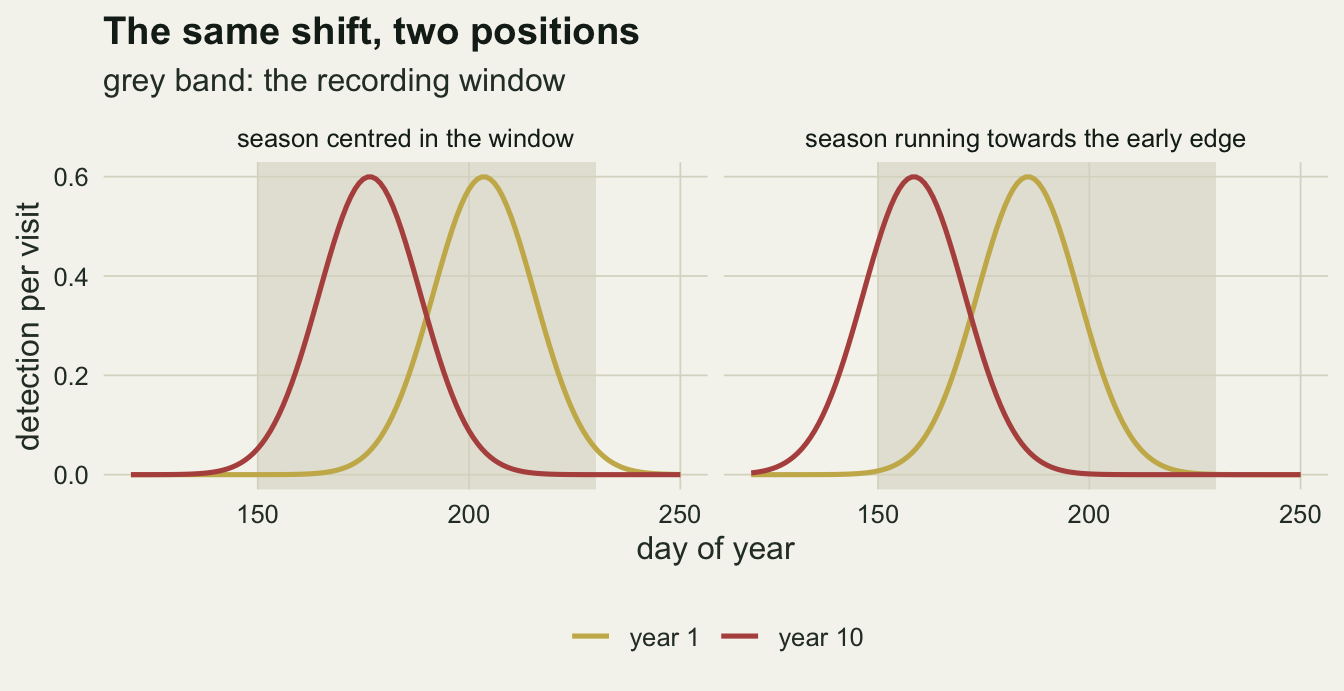
Five ways to fit the same records
Four estimators get the same simulated records, plus one alternative repair. The detected share is a logistic regression of “any detection at the site-year” on year, the analysis an occupancy model is meant to improve on. The other three, and the alternative repair, are occupancy likelihoods in the MacKenzie et al. (2002) form, with logit occupancy linear in centred year in every case, so all of them report the trend on the same scale.
The year-specific p model gives every year its own constant detection probability, which is the year-level repair of the Dail-Madsen post (logit-linear in year there), given here one free value per year. Because detection is constant within a year, the likelihood needs only the number of detections per site-year, and it is fitted from a ten by five table. The site effect variant adds a logit-normal random effect on detection, integrated with ten-point Gauss-Hermite quadrature, and lets the log of its standard deviation change linearly with year; it is the alternative repair for heterogeneity. The fixed curve model uses the visit dates: detection is a height times a Gaussian in day with one peak and one width for all years. The moving curve model lets that peak move linearly with year, which is the structure the data were generated from and a simplified, parametric version of the seasonal detectability curves in Strebel et al.
The two curve models work on the full visit-by-site-year matrix, so they get an analytic gradient, checked once against central differences away from the truth; all fits use optim with BFGS, with occupancy started from the detected share. The site effect model is started twice, once from there and once from the year-specific p estimates, and keeps the better likelihood, because a single start sometimes stopped short of the best optimum. The curve models start from the mean and standard deviation of the detection days. A start at the window centre with a generous width let some fits run off to a flat curve with a width far wider than the window, which is a constant-p model in disguise, and that local optimum is easy to miss because the fit reports convergence.
curve_parts <- function(dat, move) {
  y_mat <- dat$y
  none  <- rowSums(y_mat) == 0
  pieces <- function(th) {
    s_u   <- plogis(th[1] + th[2] * unit_yc)
    peak  <- th[4] + (if (move) th[6] else 0) * unit_yc
    sig2  <- exp(2 * th[5])
    dev   <- dat$days - peak
    log_p <- plogis(th[3], log.p = TRUE) - dev^2 / (2 * sig2)
    p_mat <- exp(log_p)
    l_occ <- exp(rowSums(y_mat * log_p + (1 - y_mat) * log1p(-p_mat)))
    list(s_u = s_u, sig2 = sig2, dev = dev, p_mat = p_mat, l_occ = l_occ,
         lik = s_u * l_occ + (1 - s_u) * none)
  }
  nll <- function(th) -sum(log(pieces(th)$lik))
  grad <- function(th) {
    pc    <- pieces(th)
    w_occ <- pc$s_u * pc$l_occ / pc$lik
    d_psi <- (pc$l_occ - none) / pc$lik * pc$s_u * (1 - pc$s_u)
    resid <- (y_mat - pc$p_mat) / (1 - pc$p_mat)
    g_m   <- rowSums(resid * pc$dev) / pc$sig2
    -c(sum(d_psi), sum(d_psi * unit_yc),
       sum(w_occ * rowSums(resid) * (1 - plogis(th[3]))),
       sum(w_occ * g_m), sum(w_occ * rowSums(resid * pc$dev^2) / pc$sig2),
       if (move) sum(w_occ * g_m * unit_yc))
  }
  det_days <- dat$days[y_mat == 1]
  list(nll = nll, grad = grad,
       start = c(psi_start(dat), 0, 0, mean(det_days), log(sd(det_days)),
                 if (move) 0))
}

psi_start <- function(dat) qlogis(max(mean(rowSums(dat$y) > 0), 0.05))

wald_out <- function(fit, hess, extra = NA) {
  cov_m <- tryCatch(solve(hess), error = function(e) NULL)
  se_b  <- if (is.null(cov_m) || cov_m[2, 2] <= 0) NA else sqrt(cov_m[2, 2])
  c(slope = fit$par[2], se = se_b, psi = plogis(fit$par[1]),
    extra = extra, conv = fit$convergence)
}

fit_curve <- function(dat, move) {
  cp  <- curve_parts(dat, move)
  fit <- optim(cp$start, cp$nll, cp$grad, method = "BFGS",
               control = list(maxit = 500))
  wald_out(fit, optimHess(fit$par, cp$nll, cp$grad),
           if (move) fit$par[6] else NA)
}

gh_nodes <- c(-3.436159, -2.532732, -1.756684, -1.036611, -0.342901,
              0.342901, 1.036611, 1.756684, 2.532732, 3.436159)
gh_wts <- c(7.640433e-06, 1.343646e-03, 3.387439e-02, 2.401386e-01,
            6.108626e-01, 6.108626e-01, 2.401386e-01, 3.387439e-02,
            1.343646e-03, 7.640433e-06) / sqrt(pi)

fit_year_p <- function(dat, site_re = FALSE) {
  n_vis <- ncol(dat$y)
  n_det <- 0:n_vis
  tab   <- matrix(table(factor(unit_yr, seq_len(n_year)),
                        factor(rowSums(dat$y), n_det)), n_year)
  nll <- function(th, re) {
    s_t <- plogis(th[1] + th[2] * year_c)
    tot <- 0
    for (yr in seq_len(n_year)) {
      if (re) {
        re_sd <- exp(th[n_year + 3] + th[n_year + 4] * year_c[yr])
        p_q   <- plogis(th[2 + yr] + sqrt(2) * re_sd * gh_nodes)
        l_occ <- vapply(n_det, function(k) sum(gh_wts * p_q^k *
                                               (1 - p_q)^(n_vis - k)), 0)
      } else {
        p_y   <- plogis(th[2 + yr])
        l_occ <- p_y^n_det * (1 - p_y)^(n_vis - n_det)
      }
      lik <- s_t[yr] * l_occ + (1 - s_t[yr]) * (n_det == 0)
      tot <- tot + sum(tab[yr, ] * log(lik))
    }
    -tot
  }
  run <- function(st, re) {
    optim(st, nll, re = re, method = "BFGS", control = list(maxit = 2000))
  }
  base_th <- c(psi_start(dat), 0, rep(0, n_year))
  fit <- run(base_th, re = FALSE)
  if (site_re) {
    # two starts, the detected share and the year-specific p optimum; keep the better
    fits <- list(run(c(base_th, log(0.5), 0), re = TRUE),
                 run(c(fit$par, log(0.5), 0), re = TRUE))
    fit <- fits[[which.min(sapply(fits, function(f) f$value))]]
  }
  # extra: for the site effect, the ratio of its sd in year 10 to year 1
  wald_out(fit, optimHess(fit$par, nll, re = site_re),
           if (site_re) exp(fit$par[n_year + 4] * (year_c[n_year] - year_c[1])) else NA)
}

fit_naive <- function(dat) {
  seen <- rowSums(dat$y) > 0
  unname(coef(glm(seen ~ unit_yc, family = binomial))[2])
}

set.seed(4101)
check_dat <- sim_records(mid_edge, shift_use, 5, n_visit_use)
check_cp  <- curve_parts(check_dat, move = TRUE)
check_th  <- c(qlogis(0.35), -0.05, qlogis(0.55), 175, log(13), -2)
num_grad  <- vapply(seq_along(check_th), function(j) {
  step <- rep(0, length(check_th))
  step[j] <- 1e-5
  (check_cp$nll(check_th + step) - check_cp$nll(check_th - step)) / 2e-5
}, 0)
grad_gap <- max(abs(num_grad - check_cp$grad(check_th)) / pmax(1, abs(num_grad)))
The grid: where the season sits, and how visits bunch
The main grid crosses the two geometries with the three visit patterns, all with a shift of 3 days a year and four visits. Each cell has 20 replicate data sets, a number fixed before the grid ran. Every mean trend below is followed in brackets by its Monte Carlo standard error, and the figure draws two of them either side.
run_cell <- function(peak_mid, clus_sd, n_rep, seed, shift = shift_use,
                     n_visit = n_visit_use, trend = 0, with_re = TRUE) {
  set.seed(seed)
  out <- lapply(seq_len(n_rep), function(r) {
    dat <- sim_records(peak_mid, shift, clus_sd, n_visit, trend)
    rbind(naive   = c(fit_naive(dat), NA, NA, NA, 0),
          year_p  = fit_year_p(dat),
          site_re = if (with_re) fit_year_p(dat, site_re = TRUE) else rep(NA, 5),
          fixed   = fit_curve(dat, move = FALSE),
          moving  = fit_curve(dat, move = TRUE))
  })
  arr <- simplify2array(out)
  dimnames(arr)[[2]] <- c("slope", "se", "psi", "extra", "conv")
  arr
}

summarise_cell <- function(arr, trend = 0) {
  n_r <- dim(arr)[3]
  data.frame(estimator = dimnames(arr)[[1]],
    slope = apply(arr[, "slope", , drop = FALSE], 1, mean),
    slope_mcse = apply(arr[, "slope", , drop = FALSE], 1, sd) / sqrt(n_r),
    psi = apply(arr[, "psi", , drop = FALSE], 1, mean),
    cover = apply(abs(arr[, "slope", , drop = FALSE] - trend) <
                    1.96 * arr[, "se", , drop = FALSE], 1, mean, na.rm = TRUE),
    row.names = NULL)
}

n_rep_grid <- 20
grid_design <- expand.grid(geometry = c("central", "edge"),
                           clus_sd = c(0, 5, 14), stringsAsFactors = FALSE)
grid_arrays <- lapply(seq_len(nrow(grid_design)), function(i) {
  run_cell(if (grid_design$geometry[i] == "central") mid_central else mid_edge,
           grid_design$clus_sd[i], n_rep_grid, seed = 5200 + i)
})
grid_tab <- do.call(rbind, lapply(seq_len(nrow(grid_design)), function(i) {
  cbind(grid_design[i, ], summarise_cell(grid_arrays[[i]]), row.names = NULL)
}))
cell_val <- function(g, cs, est, what) {
  grid_tab[grid_tab$geometry == g & grid_tab$clus_sd == cs &
             grid_tab$estimator == est, what]
}
shift_draws <- function(g, cs) {
  grid_arrays[[which(grid_design$geometry == g &
                       grid_design$clus_sd == cs)]]["moving", "extra", ]
}
n_nonconv <- sum(sapply(grid_arrays, function(a) sum(a[-1, "conv", ] != 0)))
n_se_missing <- sum(sapply(grid_arrays, function(a) sum(is.na(a[-1, "se", ]))))
n_fits_se <- 4 * n_rep_grid * nrow(grid_design)
cell_draws <- function(g, cs, est, what) {
  grid_arrays[[which(grid_design$geometry == g &
                     grid_design$clus_sd == cs)]][est, what, ]
}
The gradient check agrees to a largest relative difference of 2.51e-07. Across the grid the number of likelihood fits that reported non-convergence was 0, and 0 of 480 fits failed to give a standard error for the trend. Wald coverage from 20 replicates has a Monte Carlo standard error of 0.049 when the true coverage is 0.95, so it is a coarse check only.
With the season in the centre of the window nothing produces a trend beyond Monte Carlo error. The largest mean trend among the central cells is -0.0173, for the site effect model with visits bunched at 14 days, with a Monte Carlo standard error of 0.0107, and the year-specific p model with independent visit days gives +0.0075 (0.0048). The central geometry does show the known level bias. With visits bunched at 5 days the year-specific p model puts occupancy at 0.242 against the true 0.4, the site effect model at 0.286 and the fixed curve at 0.341, while the moving curve returns 0.402. A biased level that stays biased by the same amount every year does not make a trend.
At the edge, with independent visit days, the detected share falls at -0.0240 per year (0.0038), in line with the arithmetic value of -0.0246. The year-specific p model removes it: +0.0002 (0.0073). This is the neighbour posts’ result, and it holds here because a visit day drawn at random from the window makes every visit an independent draw from the same mixture, so the season changes detection per year and nothing else. The fixed curve does not repair it, at -0.0267 (0.0046), because one curve for all years is wrong in every year except near the middle of the series.
Bunch the visits and the year term stops working. With a 5 day spread the year-specific p model gives -0.0557 (0.0034), steeper than the detected share it was meant to correct, at -0.0451; with a 14 day spread it gives -0.0615 (0.0039). Its Wald interval covers the true zero in a share of 0.10 and 0.10 of replicates. The site effect with a year-varying spread does no better, at -0.0743 and -0.0671, with wider Monte Carlo errors. The fixed curve gives -0.0468 and -0.0449. Over ten years a slope of -0.056 on the logit scale takes occupancy of 0.4 in the middle of the series to about 0.34 in the last year and 0.46 in the first, a decline large enough to be reported as a loss of sites.
The moving curve gets the edge right in every visit pattern: +0.0019, -0.0012 and +0.0035, with coverage of 0.90, 0.95 and 1.00. Its estimate of the shift averages -2.95 days a year with visits bunched at 5 days, with a standard deviation of 0.14 across replicates, against the true -3.
est_lab <- c(naive = "detected share", year_p = "year-specific p",
             site_re = "year p + site effect", fixed = "fixed curve",
             moving = "moving curve")
vis_lab <- c("visit days independent", "visits bunched, sd 5 days",
             "visits bunched, sd 14 days")
plot_tab <- grid_tab
plot_tab$estimator <- factor(est_lab[plot_tab$estimator], levels = rev(est_lab))
plot_tab$geometry  <- factor(geom_lab[plot_tab$geometry], levels = geom_lab)
plot_tab$visits    <- factor(vis_lab[match(plot_tab$clus_sd, c(0, 5, 14))],
                             levels = vis_lab)
dodge <- position_dodge(width = 0.6)
grid_slope <- ggplot(plot_tab, aes(slope, estimator, colour = visits)) +
  geom_vline(xintercept = 0, linetype = "dashed", colour = te_body) +
  geom_errorbar(aes(xmin = slope - 2 * slope_mcse, xmax = slope + 2 * slope_mcse),
                orientation = "y", width = 0, position = dodge, linewidth = 0.6) +
  geom_point(size = 2.2, position = dodge) +
  facet_wrap(~ geometry) +
  scale_x_continuous(breaks = c(-0.1, -0.05, 0)) +
  scale_colour_manual(values = c(te_gold, te_forest, te_rust), name = NULL) +
  labs(x = "mean fitted trend in logit occupancy per year (truth 0)", y = NULL,
       title = "A false decline needs the edge and bunched visits",
       subtitle = "bars: two Monte Carlo standard errors either side") +
  theme_datasheet() + theme(legend.position = "bottom")
grid_psi <- ggplot(plot_tab[plot_tab$estimator != "detected share", ],
                   aes(psi, estimator, colour = visits)) +
  geom_vline(xintercept = psi_true, linetype = "dashed", colour = te_body) +
  geom_point(size = 2.2, position = dodge) +
  facet_wrap(~ geometry) +
  scale_colour_manual(values = c(te_gold, te_forest, te_rust), guide = "none") +
  labs(x = "mean fitted occupancy, middle of the series (truth 0.4)", y = NULL) +
  theme_datasheet()
(grid_slope / grid_psi) + plot_layout(heights = c(1.3, 1)) +
  plot_annotation(theme = theme_datasheet())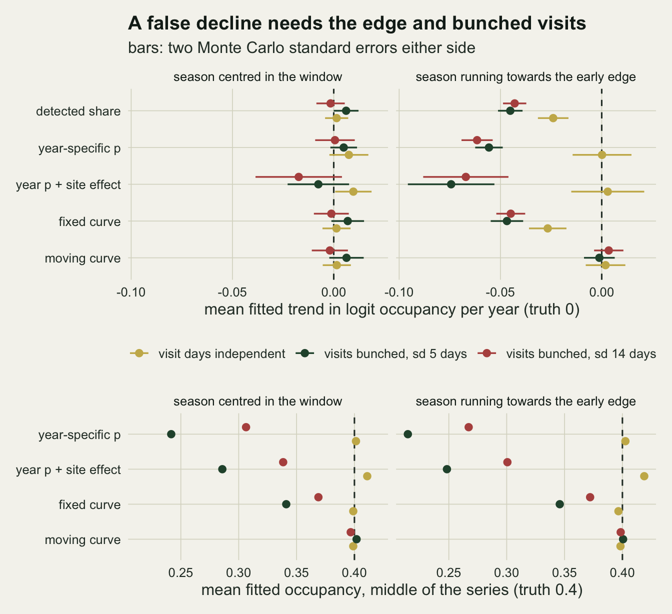
Why a year term on detection is not enough
The year-specific p model fails at the edge only when visits bunch, and the reason is heterogeneity rather than a trend in mean detection. When the four visits of a site-year fall in the same fortnight, they share that fortnight’s position in the season. A site visited at the peak has a high detection probability on every visit, a site visited in the weeks after the season has ended has almost none, and a single p per year averages over them. That is the setting of Royle (2006): unmodelled among-site variation in detection makes an occupied site that is hard to detect look like an empty one, and the constant-p estimate of occupancy comes out low.
The level bias alone does not make a trend; the trend comes from the bias changing. The chunk below computes, for the 5 day bunching and without any fitting, the expected per-visit detection of every possible site-year centre date, its coefficient of variation across sites, and the share of occupied site-years with at least one detection, both as it really is and as a single p per year would imply it.
centre_grid <- seq(win_lo, win_hi, by = 0.5)
set.seed(6130)
offset_draws <- rnorm(4000, 0, 5)
het_tab <- do.call(rbind, lapply(names(geom_lab), function(g) {
  mid_g <- if (g == "central") mid_central else mid_edge
  do.call(rbind, lapply(seq_len(n_year), function(yr) {
    peak <- mid_g + shift_use * year_c[yr]
    site_p <- vapply(centre_grid, function(cc) {
      d_v <- pmin(pmax(cc + offset_draws, win_lo), win_hi)
      mean(p_max * exp(-(d_v - peak)^2 / (2 * season_sd^2)))
    }, 0)
    p_pool <- mean(site_p)
    data.frame(geometry = g, year = yr, p_mean = p_pool,
               p_cv = sd(site_p) / p_pool,
               det_true = mean(1 - (1 - site_p)^n_visit_use),
               det_homog = 1 - (1 - p_pool)^n_visit_use)
  }))
}))
het_tab$det_ratio <- het_tab$det_true / het_tab$det_homog
het_e <- het_tab[het_tab$geometry == "edge", ]
het_c <- het_tab[het_tab$geometry == "central", ]
In the central geometry the coefficient of variation of site-level detection stays between 0.869 and 0.901 across the ten years. In the edge geometry it climbs from 0.871 in the first year to 1.261 in the last, because more and more site-years have all their visits after the flight season has finished. The ratio of the true detected share at occupied sites to the share a single p implies falls from 0.798 to 0.682 at the edge and stays between 0.785 and 0.798 in the centre. A model that allows detection to change by year but not among sites has no parameter that can follow a growing spread, so the shortfall goes into occupancy, and it grows year by year.
The site effect with a year-varying standard deviation has such a parameter, and it still failed in the grid. With four visits per site-year its fitted spread does not follow the growing heterogeneity. In the bunched edge cells the estimated standard deviation in year 10 was smaller than in year 1 in 12 of 20 fits with visits bunched at 5 days and 13 of 20 at 14 days, while the occupancy trend absorbed the change: the per-fit trends at 5 days run from -0.162 to +0.009, against -0.083 to -0.016 for the year-specific p model. The moving curve does not need to describe the heterogeneity at all, because it conditions on the visit dates that cause it.
het_plot <- het_tab
het_plot$geometry <- factor(geom_lab[het_plot$geometry], levels = geom_lab)
ggplot(het_plot, aes(year, det_ratio, colour = geometry)) +
  geom_hline(yintercept = 1, linetype = "dashed", colour = te_body) +
  geom_line(linewidth = 0.9) + geom_point(size = 2) +
  scale_colour_manual(values = c(te_forest, te_rust), name = NULL) +
  scale_x_continuous(breaks = 1:n_year) +
  labs(x = "year", y = "true over one-p value", title = "Detected share, occupied",
       subtitle = "true share over what one p implies, visits bunched, sd 5 days") +
  theme_datasheet() + theme(legend.position = "bottom")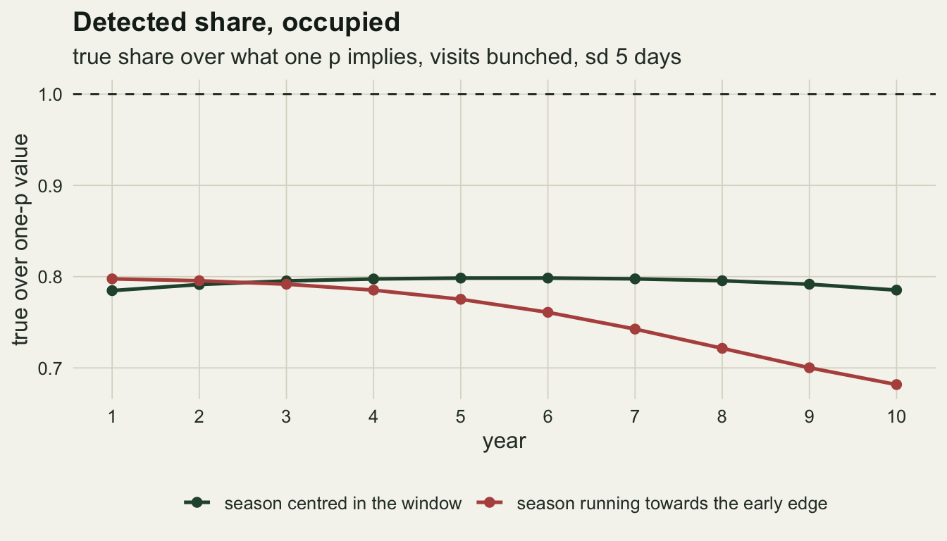
More visits, a smaller shift, a real decline
Three arms vary one design choice at a time around the edge geometry with visits bunched at 5 days: the number of visits per site-year (2 and 8 besides 4), the size of the shift (0 and 1.5 days a year besides 3), and a real decline of -0.04 per year on the logit scale. The site effect model is left out of the arms to keep the run short. Each new cell again has 20 replicates.
n_rep_arm <- 20
edge5 <- grid_arrays[[which(grid_design$geometry == "edge" &
                              grid_design$clus_sd == 5)]]
arm_visits <- lapply(c(2, 8), function(k)
  run_cell(mid_edge, 5, n_rep_arm, seed = 7300 + k, n_visit = k, with_re = FALSE))
arm_shift <- lapply(c(0, -1.5), function(sh)
  run_cell(mid_edge, 5, n_rep_arm, seed = 7400 + 10 * abs(sh), shift = sh,
           with_re = FALSE))
trend_decl <- -0.04
arm_trend <- run_cell(mid_edge, 5, n_rep_arm, seed = 7500, trend = trend_decl,
                      with_re = FALSE)

arm_tab <- rbind(
  cbind(arm = "visits", level = 2, summarise_cell(arm_visits[[1]])),
  cbind(arm = "visits", level = 4, summarise_cell(edge5)),
  cbind(arm = "visits", level = 8, summarise_cell(arm_visits[[2]])),
  cbind(arm = "shift", level = 0, summarise_cell(arm_shift[[1]])),
  cbind(arm = "shift", level = -1.5, summarise_cell(arm_shift[[2]])),
  cbind(arm = "shift", level = -3, summarise_cell(edge5)))
trend_tab <- summarise_cell(arm_trend, trend = trend_decl)
arm_val <- function(a, lv, est, what) {
  arm_tab[arm_tab$arm == a & arm_tab$level == lv & arm_tab$estimator == est, what]
}
tr_val <- function(est, what) trend_tab[trend_tab$estimator == est, what]
shift_trend <- arm_trend["moving", "extra", ]
More visits do not wash the bias out. The year-specific p trend is -0.0541 with two visits, -0.0557 with four and -0.0577 with eight, and the fixed curve goes from -0.0421 to -0.0517. Extra visits inside the same fortnight measure the same position in the season more precisely; they do not add information about the part of the season the recorder missed. The year-specific p interval covers zero in 0.05 of replicates with eight visits, so the added precision makes the false decline easier to call significant. The moving curve stays at -0.0010, -0.0012 and +0.0028.
The false trend scales with the shift. With no shift every estimator is flat, the largest mean trend being -0.0026 (0.0063) for the fixed curve, which in that cell is the correct model. With a shift of 1.5 days a year the year-specific p model gives -0.0283, 0.51 of its value at 3 days a year. In that arm the no-shift cell also shows the year-specific p model’s level bias without any trend: occupancy 0.223.
When occupancy really declines at -0.04 per year, the moving curve returns -0.0404 (0.0046) with coverage 0.90 and a shift estimate averaging -3.03 days a year. The year-specific p model reports -0.0871 and the fixed curve -0.0832, so the false decline adds to the real one and the reported decline is about 2.2 times the truth. A real decline and a season sliding off the window are not confused by the moving curve; they are confused by the other two.
What to report
State the recording window and where the species’ flight season sits in it, year by year if the data allow. The grid says the geometry decides the size of the problem: the same three-day-a-year advance produced no trend in the centre of the window and a decline of -0.056 per year on the logit scale at the edge. A plot of detection days by year against the window edges is the cheapest diagnostic there is, and it is the one a referee will ask for.
Report how visits are spread within a site-year, for example the median range of visit dates per site. If visit days are close to independent of the site, a year term on detection handles a moving season; if a site’s visits bunch, it does not, and quoting a year effect on p as the detection correction is then not enough.
Fit detection as a function of visit date with a peak that is allowed to move with year, and report the estimated shift with its standard error beside the occupancy trend. If the shift is near zero the fixed curve and the moving curve agree and nothing is lost. Start the curve from the detection days rather than from a guess, and compare the log-likelihood with a year-specific p fit: a curve fit whose width is many times the window has fallen into the flat solution. More bunched visits per site-year do not replace this.
Honest limits
Detection here is a single symmetric Gaussian with constant height and width. A real flight season can be skewed, can have two broods, and can change in length over the years, as Roth et al. report for the flight periods of some butterflies; a moving peak with a fixed width would then be misspecified in its own way, and none of that was simulated. The Strebel et al. curve is more flexible than the one fitted here.
The shift is linear in year and known in form to the moving curve model. Real phenology tracks spring temperature and jumps between years. A curve whose peak follows a year-specific value, or a temperature covariate, would be the natural model and was not tested.
Occupancy is constant, closed within each site-year, and independent across years at the same site. The butterfly on a real site is the same colony next year, so a dynamic occupancy model would be the realistic trend model, and the detection problem would sit in the same place in it, but the sizes above were not measured there. The bunched visits come from one mechanism, a uniform centre date per site-year with normal scatter clamped at the window edges, which puts visits on the first and last day of the window more often than real recorders would. Recorders who choose their visit dates to match the season, going out earlier when the season is early, would reduce the problem, and recorders who stick to their holidays would not; the simulation assumes the second.
The grid has 20 replicates per cell, which resolves trends of the size reported but not differences of a few thousandths or coverage differences of less than about ten percentage points. The site effect model tried here is one form of heterogeneity model; a finite mixture on detection or a Royle-Nichols model puts the heterogeneity in a different form, and neither was fitted.
References
MacKenzie DI, Nichols JD, Lachman GB, Droege S, Royle JA, Langtimm CA 2002 Ecology 83(8):2248-2255 (10.1890/0012-9658(2002)083[2248:ESORWD]2.0.CO;2)
Royle JA 2006 Biometrics 62(1):97-102 (10.1111/j.1541-0420.2005.00439.x)
Strebel N, Kery M, Schaub M, Schmid H 2014 Methods in Ecology and Evolution 5(5):483-490 (10.1111/2041-210X.12175)
Roth T, Strebel N, Amrhein V 2014 Ecology 95(8):2144-2154 (10.1890/13-1830.1)
van Strien AJ, van Swaay CAM, Termaat T 2013 Journal of Applied Ecology 50(6):1450-1458 (10.1111/1365-2664.12158)