library(ggplot2)

te_paper  <- "#f5f4ee"
te_ink    <- "#16241d"
te_body   <- "#2c3a31"
te_forest <- "#275139"
te_rust   <- "#b5534e"
te_gold   <- "#c9b458"
te_line   <- "#dad9ca"

theme_datasheet <- function() {
  theme_minimal(base_size = 12) +
    theme(plot.background  = element_rect(fill = te_paper, colour = NA),
          panel.background = element_rect(fill = te_paper, colour = NA),
          panel.grid.major = element_line(colour = te_line, linewidth = 0.3),
          panel.grid.minor = element_blank(),
          text             = element_text(colour = te_body),
          plot.title       = element_text(colour = te_ink, face = "bold"),
          axis.text        = element_text(colour = te_body))
}
Daylength as a predictor in ecology
R
phenology
photoperiod
simulation
ecology tutorial
Compute photoperiod in base R and test it: at one site daylength cannot beat day of year for phenology, and across latitudes it carries the climate gradient.
Corrected 30 September 2026: the closing sections said a day and its reflection differ in daylength by fractions of a second, that Forsythe et al compared daylength models rather than proposing one, and that daylength is missing where the sun never sinks to the reference angle; they now say the gap is minutes, that Forsythe et al proposed and recommended this model, and that daylength there is a full day.
Corrected 27 September 2026: the residual section said a photoperiod model fitted to a lagged response is systematically low in spring and high in autumn; its own residuals show the reverse, and it now says the model predicts too high in spring and too low in autumn.
Day of year is the predictor everyone starts with and nobody defends. It is a calendar label, and no organism reads a calendar, so sooner or later a reviewer asks for something mechanistic. Daylength is the usual answer. Plants and insects really do measure photoperiod, the physiology behind it has been worked out in detail, and the covariate can be computed from latitude and date alone with no station data. It looks like a free upgrade.
It is not free, and within a single site it is not an upgrade either. Daylength at a fixed latitude is a deterministic function of day of year, so any smooth of day of year already contains it; and because it rises and falls symmetrically about the solstices, the same daylength arrives twice a year on two very different days. This post builds the covariate from scratch in base R, measures what it costs in a single-site model, and then shows the one design where the coefficient becomes estimable at all, along with what that coefficient is really made of.
Daylength in a dozen lines of base R
The model is the CBM (Campbell and Norman, revised) formulation compared and recommended by Forsythe et al (1995). Solar declination comes from day of year through a closed-form approximation to the orbit, the hour angle of sunrise follows from declination and latitude, and daylength is twice that angle converted to hours. There is one tuning constant, p, the angle of the sun below the horizon that counts as sunrise: 0 for the geometric centre of the disc, 0.8333 for the standard sunrise and sunset with refraction and the upper limb, 6 for civil twilight, 18 for astronomical twilight.
sun_arg <- function(doy, lat, p = 0.8333) {
  theta <- 0.2163108 + 2 * atan(0.9671396 * tan(0.00860 * (doy - 186)))
  phi   <- asin(0.39795 * cos(theta))
  (sin(p * pi / 180) + sin(lat * pi / 180) * sin(phi)) /
    (cos(lat * pi / 180) * cos(phi))
}

daylength <- function(doy, lat, p = 0.8333) {
  arg <- sun_arg(doy, lat, p)
  arg[abs(arg) > 1] <- NA      # above 1 the sun never sinks to p below the
  24 - (24 / pi) * acos(arg)   # horizon; below -1 it never climbs to it
}

all_days <- 1:365
cross12  <- function(lat, p, window)
  uniroot(function(d) daylength(d, lat, p) - 12, window)$root
eq_geom  <- range(daylength(all_days, 0, p = 0)); march_eq <- cross12(47, 0, c(60, 100))
up12     <- sapply(c(47, 65), cross12, p = 0.8333, window = c(60, 100))
down12   <- sapply(c(47, 65), cross12, p = 0.8333, window = c(240, 300))
round(c(equator_geometric_min = eq_geom[1], equator_geometric_max = eq_geom[2],
        equator_standard = daylength(1, 0), geometric_equinox = march_eq,
        day_80_at_47N = daylength(80, 47, p = 0), up12_47N = up12[1],
        up12_65N = up12[2], down12_47N = down12[1], down12_65N = down12[2]), 3)
equator_geometric_min equator_geometric_max equator_standard
12.000 12.000 12.121
geometric_equinox day_80_at_47N up12_47N
80.208 11.988 77.326
up12_65N down12_47N down12_65N
77.883 269.576 269.012 Two checks before trusting it. At the equator with the geometric coefficient the function returns 12.000 hours on every day of the year, which is what the geometry demands, and the flatness is what Figure 1 shows. That same coefficient puts the March equinox, the day the curve crosses twelve hours, at day 80.21; on day 80 at 47 degrees north the function returns 11.988 hours, 42 seconds short of twelve. Switching to the standard coefficient lifts the equator to 12.12 hours, because refraction and the width of the solar disc add a few minutes at both ends of the day everywhere.
curve_df <- expand.grid(doy = all_days, lat = c(0, 47, 65))
curve_df$hours <- daylength(curve_df$doy, curve_df$lat)
curve_df$site  <- paste(curve_df$lat, "degrees north")

ggplot(curve_df, aes(doy, hours, colour = site)) +
  geom_hline(yintercept = 12, linetype = "dashed", colour = te_body) +
  geom_line(linewidth = 1) +
  scale_colour_manual(values = c(te_gold, te_forest, te_rust)) +
  labs(x = "day of year", y = "daylength (hours)", colour = NULL,
       title = "The covariate the model actually sees") +
  theme_datasheet() +
  theme(legend.position = "bottom")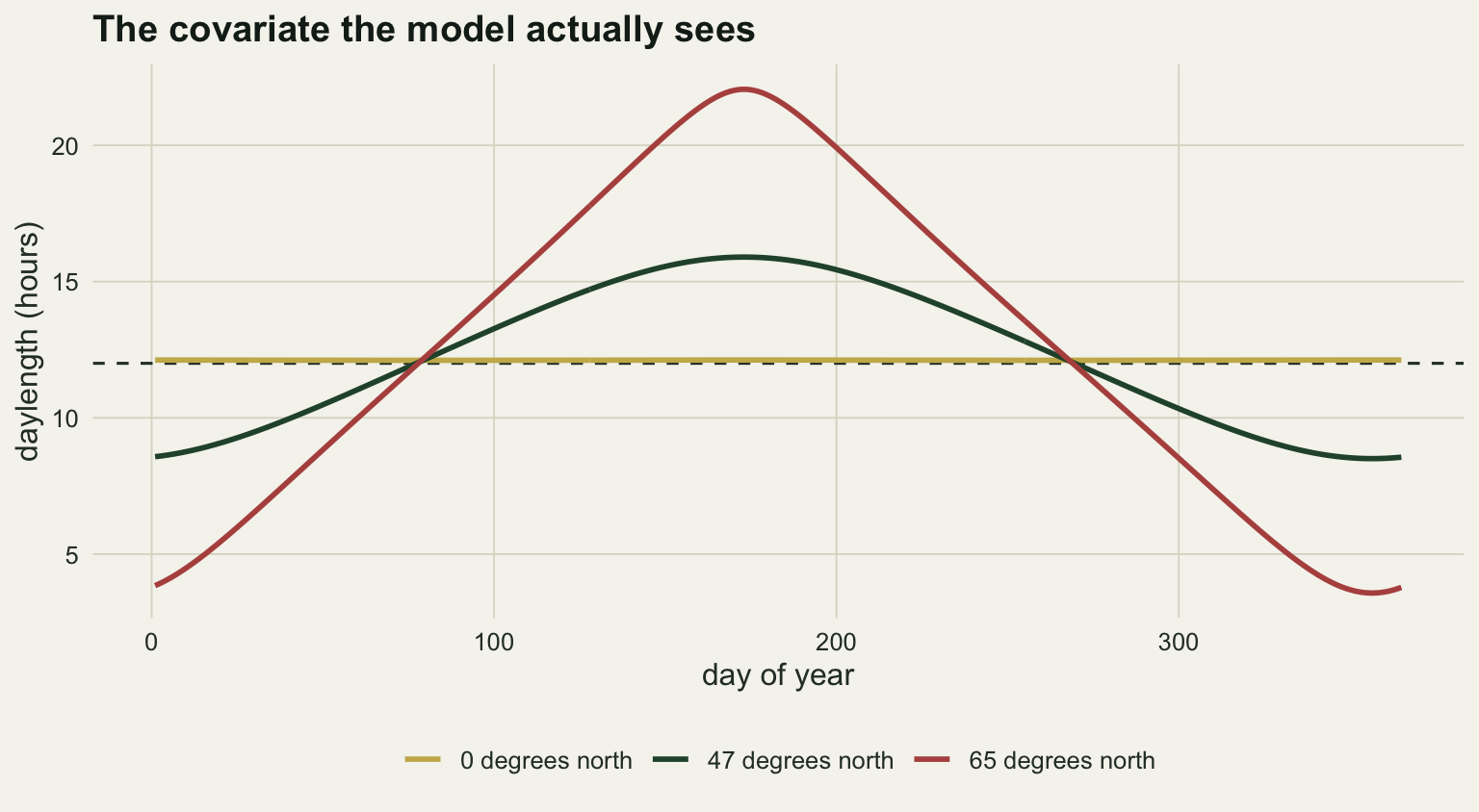
At 47 degrees north the annual swing is 7.39 hours and at 65 degrees north it is 18.48 hours. The two curves look as though they cross twelve hours on the same two days, and under the geometric coefficient they would: day 80.21 in March, and its September counterpart, at every latitude, because the equinox belongs to the orbit and not to the observer. Under the standard coefficient they do not. Refraction and the upper limb buy more extra daylight where the sun crosses the horizon at a shallower angle, so both sites reach twelve hours before the March equinox and leave it after the September one: day 77.3 and day 269.6 at 47 degrees north, against day 77.9 and day 269.0 at 65. The separation is under a day here, and it is the same tuning constant that turns up later as a real problem.
Within one site it is day of year in other units
Fix the latitude and the function above has one argument left. Daylength is then a smooth, deterministic transform of day of year, and a regression cannot tell the two apart. The measurement below is the one that matters for model building: how much of the daylength covariate is already inside a seasonal basis built from day of year alone. Two harmonics is a modest basis, four columns, the sort of thing anybody would use for a seasonal term.
harmonics <- function(d, k) do.call(cbind, lapply(1:k, function(j)
  cbind(sin(2 * pi * j * d / 365), cos(2 * pi * j * d / 365))))

lat_site <- 47
doy <- seq(32, 335, by = 3)
dl <- daylength(doy, lat_site); H2 <- harmonics(doy, 2)

r2_alias <- summary(lm(dl ~ H2))$r.squared
r2_three <- summary(lm(dl ~ harmonics(doy, 3)))$r.squared
round(c(n_days = length(doy), r2_on_two_harmonics = r2_alias,
        variance_inflation = 1 / (1 - r2_alias),
        r2_on_three_harmonics = r2_three), 6)
n_days r2_on_two_harmonics variance_inflation
102.000000 0.999122 1138.826372
r2_on_three_harmonics
0.999998 Two harmonics of day of year explain 0.9991 of the variance in daylength at this site. Put both in the same model and the variance inflation factor on the daylength coefficient is 1139, which is not a borderline collinearity problem; it is an aliasing problem wearing a collinearity label, and it gets worse, not better, as the seasonal basis is made more flexible. Three harmonics take the shared variance to 0.999998. The general diagnostics for this situation are in collinearity and VIF; what is unusual here is that the two predictors are not correlated by accident of sampling but by construction, so no amount of extra data will separate them.
The second property is the one that costs something. Daylength rises to the June solstice and falls away from it, so almost every value occurs twice: once in spring and once in autumn. Inverting each monotone branch numerically gives each day its mirror, the day on the other side of the solstice with the same daylength. The rising branch runs across the turn of the year, so it has to be unwrapped past day 365 before it is interpolated and folded back afterwards; interpolate on a branch that jumps from 365 to 1 and the mirror comes back in the wrong half of the year.
dl_grid <- daylength(all_days, lat_site)
day_max <- which.max(dl_grid); day_min <- which.min(dl_grid)
fall_days <- day_max:day_min                     # daylength decreasing
rise_days <- day_min:(365 + day_max)             # daylength increasing
rise_dl   <- daylength(((rise_days - 1) %% 365) + 1, lat_site)

mirror_day <- function(d) {
  target <- daylength(d, lat_site)
  m <- ifelse(d > day_max & d < day_min,
              approx(rise_dl, rise_days, xout = target)$y,
              approx(dl_grid[fall_days], fall_days, xout = target)$y)
  ((m - 1) %% 365) + 1
}

example <- c(116, 347)
round(cbind(day = example, mirror = mirror_day(example),
            hours = daylength(example, lat_site),
            hours_at_mirror = daylength(mirror_day(example), lat_site)), 3)
day mirror hours hours_at_mirror
[1,] 116 230.371 14.125 14.125
[2,] 347 365.723 8.569 8.566Day 116, in late April, and day 230.4, in the third week of August, share a daylength of 14.12 hours to within 0.1 seconds. The second row is the case that breaks a naive implementation: day 347 sits in December on the falling branch, and its mirror is day 365.7, at the very end of the same year. Any model whose only seasonal predictor is daylength is required to give a day and its mirror the same fitted value. Whether that is acceptable depends entirely on whether the response is symmetric about the solstice, and for most temperate responses it is not, because temperature is not.
The cost: the same daylength happens twice
Here is a single site, 102 sampling days spread from the first of February to the first of December, and a response driven by temperature. Temperature at a mid-latitude site lags the sun: the ground and the air are still warming after the June solstice, so the thermal peak arrives in late July. That lag is the whole mechanism, and it is enough to make the response asymmetric about the solstice while daylength stays symmetric.
lag_days     <- 32
thermal_peak <- day_max + lag_days                        # late July
site_temp <- function(d, peak = thermal_peak) 9 + 11 * cos(2 * pi * (d - peak) / 365)
mu_true   <- function(d, peak = thermal_peak) 6 + 0.9 * site_temp(d, peak)

set.seed(20260813)
noise <- rnorm(length(doy), 0, 2.2); activity <- mu_true(doy) + noise
round(c(solstice = day_max, thermal_peak = thermal_peak,
        temp_min = min(site_temp(doy)), temp_max = max(site_temp(doy)),
        response_sd = sd(activity)), 2)
solstice thermal_peak temp_min temp_max response_sd
173.00 205.00 -1.85 20.00 6.73 The response is an activity index, and nothing about it is subtle: it tracks temperature exactly, with noise. Now fit it twice on the same values, once against a flexible function of daylength and once against a seasonal basis in day of year with the same number of parameters. A fourth-order polynomial in daylength and two harmonics of day of year both cost five coefficients, so neither model is handed extra freedom. The same comparison is then repeated with the thermal peak moved, on the one noise draw, to show what the penalty is a penalty for.
fit_dl  <- lm(activity ~ poly(dl, 4))
fit_doy <- lm(activity ~ H2)
lags <- c(0, 12, lag_days, 47)
loss <- sapply(lags, function(L) {
  a <- mu_true(doy, peak = day_max + L) + noise
  summary(lm(a ~ H2))$r.squared - summary(lm(a ~ poly(dl, 4)))$r.squared })

round(c(r2_dl = summary(fit_dl)$r.squared, r2_doy = summary(fit_doy)$r.squared,
        sigma_dl = summary(fit_dl)$sigma, sigma_doy = summary(fit_doy)$sigma), 3)
r2_dl r2_doy sigma_dl sigma_doy
0.591 0.903 4.389 2.139 round(setNames(loss, paste0("loss_at_lag_", lags)), 3) loss_at_lag_0 loss_at_lag_12 loss_at_lag_32 loss_at_lag_47
-0.001 0.042 0.312 0.566 loop_df <- data.frame(dl = dl, activity = activity,
half = factor(ifelse(doy <= day_max, "before the solstice", "after the solstice"),
levels = c("before the solstice", "after the solstice")))
fit_df <- data.frame(dl = dl, fitted = fitted(fit_dl))
p_loop <- ggplot(loop_df, aes(dl, activity)) +
geom_point(aes(colour = half), size = 2.4, alpha = 0.85) +
geom_line(data = fit_df, aes(dl, fitted), colour = te_ink, linewidth = 1) +
scale_colour_manual(values = c(te_forest, te_rust)) +
labs(x = "daylength (hours)", y = "activity index", colour = NULL,
title = "One daylength, two answers") +
theme_datasheet() +
theme(legend.position = "bottom")
p_loop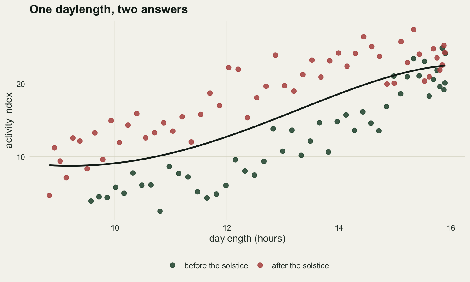
The daylength model reaches an R-squared of 0.591 and the day-of-year model 0.903, on the same 102 observations with the same 5 parameters. Residual standard deviation is 4.39 against 2.14, so the daylength model’s errors are about 2.1 times larger. The mechanistic covariate has not merely failed to help; it has thrown away roughly a third of the explained variance. All of that is the lag: put the thermal peak back on the solstice and the two models are level, with a difference of -0.001 in R-squared in the daylength model’s favour, while twelve days of lag costs 0.042, the 32 days used here cost 0.312, and a 47-day lag costs 0.566. The deficiency is structural, not a shortage of degrees of freedom, and it can be measured on the true mean curve with the noise taken out. A predictor that is symmetric about the solstice cannot separate a day from its reflection, so the best it can do is predict the average of the two true means; the half-difference between them is out of reach.
mu_year   <- mu_true(all_days)
reflected <- ((2 * day_max - all_days - 1) %% 365) + 1   # exact, and closed on 1:365
mu_refl   <- mu_true(reflected)
pair_mean <- (mu_year + mu_refl) / 2; gap <- max(abs(mu_year - mu_refl))
ceiling_r2 <- 1 - sum((mu_year - pair_mean)^2) / sum((mu_year - mean(mu_year))^2)
attained <- sapply(c(4, 20), function(k)
  summary(lm(mu_year ~ poly(dl_grid, k)))$r.squared)
round(c(r2_symmetric_ceiling = ceiling_r2, r2_poly4 = attained[1],
        r2_poly20 = attained[2], largest_reflected_gap = gap,
        sd_of_true_mean = sd(mu_year), gap_in_sd_units = gap / sd(mu_year)), 3)
r2_symmetric_ceiling r2_poly4 r2_poly20
0.726 0.732 0.732
largest_reflected_gap sd_of_true_mean gap_in_sd_units
10.364 7.010 1.478 Reflecting the year about the solstice and averaging each pair leaves 0.726 of the variance in the true mean, and that is the ceiling for any predictor forced to treat a day and its reflection alike. Flexibility is not the missing ingredient: a fourth-order polynomial in daylength reaches 0.732, and raising the order to twenty returns 0.732, the same figure to three decimals. Both sit 0.006 above the symmetric ceiling rather than below it, and that margin is the whole of what the orbit buys: daylength is not quite symmetric about the solstice, so a function of it is held very close to the ceiling rather than strictly under it. The largest gap between a day and its reflection is 10.4 units of the response against a seasonal standard deviation of 7.0, so two days a symmetric predictor cannot tell apart differ by 1.48 seasonal standard deviations. That failure has a signature, and it is easy to look for in a real fit.
res_dl <- resid(fit_dl); res_doy <- resid(fit_doy)
spring <- doy <= day_max
res_df <- data.frame(doy = doy, resid = c(res_dl, res_doy),
  model = rep(c("response ~ poly(daylength, 4)",
                "response ~ two harmonics of day of year"), each = length(doy)))
seg_df <- do.call(rbind, lapply(split(res_df, list(res_df$model, res_df$doy <= day_max)),
  function(z) data.frame(model = z$model[1], x = min(z$doy),
                         xend = max(z$doy), y = mean(z$resid))))

ggplot(res_df, aes(doy, resid)) +
  geom_hline(yintercept = 0, colour = te_body) +
  geom_vline(xintercept = day_max, linetype = "dashed", colour = te_gold) +
  geom_point(colour = te_forest, size = 1.9, alpha = 0.8) +
  geom_segment(data = seg_df, aes(x = x, xend = xend, y = y, yend = y),
               colour = te_rust, linewidth = 1.4) +
  facet_wrap(~ model, ncol = 1) +
  labs(x = "day of year", y = "residual",
       title = "The daylength model is wrong in opposite directions") +
  theme_datasheet()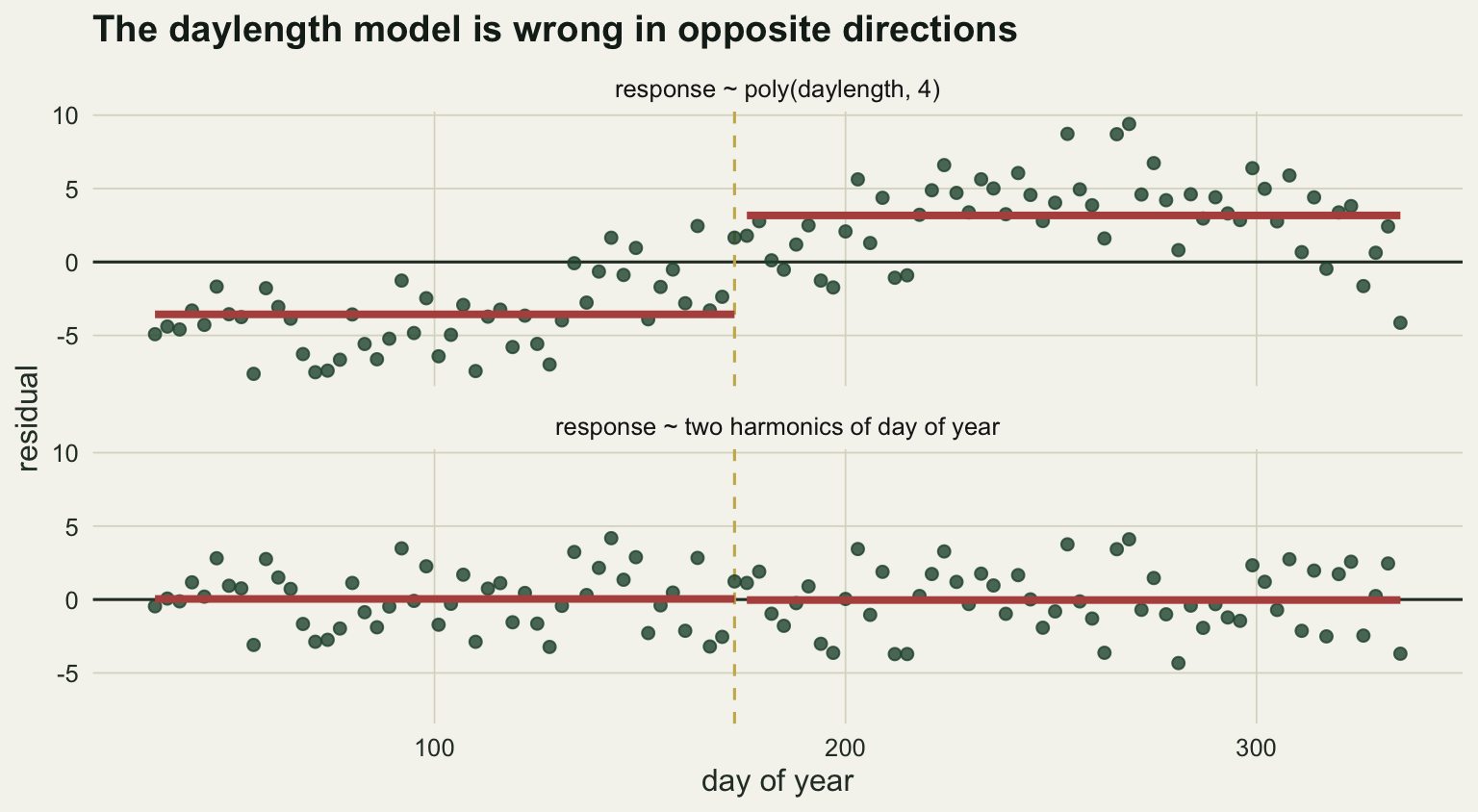
The daylength model’s residuals average -3.57 before the solstice and 3.17 after it. The day-of-year model’s averages are 0.04 and -0.04, which is nothing. A photoperiod model fitted to a lagged response predicts systematically too high in spring and systematically too low in autumn, and that sign flip is the diagnostic worth plotting before anything else.
Across latitudes the aliasing breaks
Everything above depends on latitude being fixed. Let it vary and daylength stops being a function of day of year alone: on a given date, sites at different latitudes see different daylengths, and the aliasing that made the single-site coefficient meaningless is gone.
lats    <- seq(38, 62, by = 4)
dgrid   <- seq(60, 300, by = 6); may_day <- 121
sites <- expand.grid(doy = dgrid, lat = lats)
sites$dl <- daylength(sites$doy, sites$lat); sites$site <- factor(sites$lat)
Hs <- harmonics(sites$doy, 2)

focal      <- sites[sites$lat == 46, ]
r2_focal   <- summary(lm(focal$dl ~ harmonics(focal$doy, 2)))$r.squared
r2_pool    <- summary(lm(sites$dl ~ Hs + sites$site))$r.squared
spread_may <- diff(range(daylength(may_day, lats)))
round(c(n_total = nrow(sites), spread_on_1_may = spread_may,
        r2_at_46N = r2_focal, vif_at_46N = 1 / (1 - r2_focal),
        r2_pooled = r2_pool, vif_pooled = 1 / (1 - r2_pool)), 4)
n_total spread_on_1_may r2_at_46N vif_at_46N r2_pooled
287.0000 2.5273 0.9996 2627.3170 0.9093
vif_pooled
11.0270 ggplot(sites, aes(doy, dl, colour = lat, group = lat)) +
geom_vline(xintercept = may_day, linetype = "dashed", colour = te_body) +
geom_line(linewidth = 0.9) +
scale_colour_gradient(low = te_gold, high = te_ink,
name = "latitude (degrees north)") +
labs(x = "day of year", y = "daylength (hours)",
title = "Latitude is what makes the coefficient estimable") +
theme_datasheet() +
theme(legend.position = "bottom")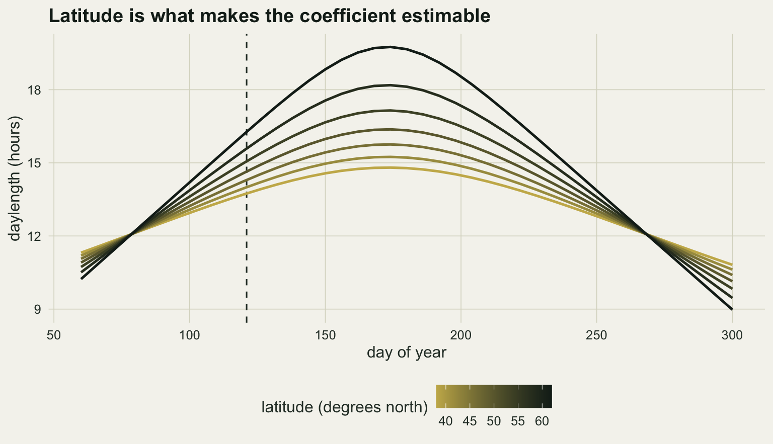
Seven sites from 38 to 62 degrees north, sampled every 6 days. On 1 May, day 121, daylength across them spans 2.53 hours. The before-and-after comparison has to hold the design fixed, so both figures come from this grid: at 46 degrees north, the site the pooled fit is checked against below, two harmonics of day of year explain 0.9996 of the variance in daylength, a variance inflation factor of 2627. Adding the other six sites and a site intercept takes the shared variance to 0.909 and the inflation factor to 11, an ordinary collinearity of the kind a design can live with. The single-site value here is worse than the 1139 of the first section because this grid samples a narrower window of the year, which only sharpens the point.
The consequence for estimation is easiest to see by generating a response that genuinely does depend on photoperiod, on top of a seasonal term shared by all sites and a site intercept, and asking each design to recover the coefficient.
beta_dl  <- 1.5
seasonal <- function(d) 8 * sin(2 * pi * (d - 100) / 365) +
                        3 * cos(2 * pi * 2 * (d - 40) / 365)
sites$mu <- 10 + beta_dl * sites$dl + seasonal(sites$doy)

set.seed(4711)
sites$y <- sites$mu + rnorm(nrow(sites), 0, 2.5)

fit_pool <- lm(y ~ dl + Hs + site, data = sites)
one_site <- sites[sites$lat == 46, ]; H_one <- harmonics(one_site$doy, 2)
fit_one  <- lm(y ~ dl + H_one, data = one_site)
ci_one   <- confint(fit_one)["dl", ]; ci_pool <- confint(fit_pool)["dl", ]
round(rbind(
  one_site    = c(coef(fit_one)["dl"], ci_one, sigma = summary(fit_one)$sigma),
  seven_sites = c(coef(fit_pool)["dl"], ci_pool, sigma = summary(fit_pool)$sigma)), 3)
dl 2.5 % 97.5 % sigma
one_site -2.590 -23.841 18.661 2.149
seven_sites 1.456 1.046 1.867 2.397The truth is 1.5 response units per hour of daylength. From one site the estimate is -2.59 with a confidence interval running from -23.8 to 18.7, a width of 42.5 units per hour. It contains the truth, and it also contains zero, twice the truth and the opposite sign; it rules out nothing. Pooling the seven sites gives 1.46 with an interval of 1.05 to 1.87, 52 times narrower and comfortably around the true 1.5. Sample size is not what did that. The pooled fit has 287 observations against 41, 7.0 times as many, and observations on their own buy the square root of that, a factor of 2.6. The observed factor is 52, and it is not bought with a quieter fit either: the pooled residual standard deviation, 2.40, is no smaller than the single-site one. The rest of the gain is latitude.
What that coefficient is actually made of
The design that makes the coefficient estimable is the design that makes it uninterpretable. Latitude does not vary on its own. Mean temperature falls towards the pole, the seasonal swing widens, the growing season shortens, the community changes. Any of those, if it acts on the response and is not fully absorbed by the site intercept, will be attributed to daylength. The demonstration is the same model on data with a photoperiod coefficient of exactly zero: the response depends only on temperature, and temperature does what temperature does with latitude, its annual mean falling and its seasonal amplitude widening towards the pole.
amp <- 1.64 + 0.22 * sites$lat
sites$temp <- (26 - 0.38 * sites$lat) +
              amp * cos(2 * pi * (sites$doy - thermal_peak) / 365)
sites$mu_no_photo <- 4 + 0.9 * sites$temp

set.seed(99001)
sites$y_no_photo <- sites$mu_no_photo + rnorm(nrow(sites), 0, 2.5)

coef_conf   <- summary(lm(y_no_photo ~ dl + Hs + site, data = sites))$coefficients["dl", ]
b_noiseless <- coef(lm(mu_no_photo ~ dl + Hs + site, data = sites))["dl"]
std_spurious <- b_noiseless * sd(sites$dl) / sd(sites$mu_no_photo)
std_genuine  <- beta_dl * sd(sites$dl) / sd(sites$mu)
round(c(amplitude_south = min(amp), amplitude_north = max(amp),
        estimate = coef_conf[1], std_error = coef_conf[2], p_value = coef_conf[4],
        noiseless_estimate = b_noiseless, standardised_spurious = std_spurious,
        standardised_genuine = std_genuine), 4)
amplitude_south amplitude_north estimate.Estimate
10.0000 15.2800 0.7520
std_error.Std. Error p_value.Pr(>|t|) noiseless_estimate.dl
0.2282 0.0011 0.8447
standardised_spurious.dl standardised_genuine
0.2875 0.4507 The seasonal amplitude runs from 10.0 degrees at the southern site to 15.3 at the northern one. There is no photoperiod effect anywhere in that simulation, and the fitted daylength coefficient is 0.75 units per hour with a standard error of 0.23, giving a p-value of 0.0011. It is not an accident of this noise draw: the same fit run on the noiseless mean returns 0.84, which is what the design itself puts there. Site intercepts absorbed the difference in mean temperature between sites; what they could not absorb is that seasonality itself strengthens towards the pole, in temperature and in daylength alike, and the model had one covariate available to carry it. On a standardised scale, with the noise out of both, the spurious coefficient is 0.29 against 0.45 for the genuine photoperiod effect of the previous section, about 64 per cent of a real effect, manufactured out of climate.
Nothing in the output distinguishes the two fits. Both give a positive coefficient with a small p-value on a covariate computed from an astronomical formula, and only the simulation code says which one means anything. What would actually identify photoperiod is a manipulation: growth chambers or field light supplementation, where daylength moves and temperature does not, which is how photoperiodic response curves are measured in the first place (Bradshaw and Holzapfel 2007). Latitudinal clines in those responses exist and are informative, but they are read against exactly this confound rather than in place of it (Hut et al 2013). Short of that, sites matched on climate but separated in latitude get part of the way, and so does a within-site design that exploits a response to daylength change rather than daylength level. An observational latitude gradient with a photoperiod label on the x-axis is a latitude gradient.
Two practical traps
The first is the twilight coefficient, which looks like a detail and is not. At the peak of the year at 47 degrees north, daylength is 15.70 hours measured to the centre of the disc, 15.90 to the standard sunrise, and 17.23 to the end of civil twilight.
civil_gap <- mean(daylength(all_days, lat_site, p = 6) - dl_grid)
disc_gap  <- mean(dl_grid - daylength(all_days, lat_site, p = 0))
undefined <- function(lat, p) {
  a <- sun_arg(all_days, lat, p)
  c(never_ends = sum(a > 1), never_starts = sum(a < -1))
}
polar <- sapply(c(62, 66.5, 68), function(L)
  c(standard = undefined(L, 0.8333), civil = undefined(L, 6)))
colnames(polar) <- paste0("lat_", c(62, 66.5, 68))
round(c(mean_civil_minus_standard = civil_gap,
        mean_standard_minus_disc = disc_gap,
        as_fraction_of_latitude_spread = civil_gap / spread_may), 3)
mean_civil_minus_standard mean_standard_minus_disc
1.126 0.180
as_fraction_of_latitude_spread
0.445 polar lat_62 lat_66.5 lat_68
standard.never_ends 0 31 52
standard.never_starts 0 0 25
civil.never_ends 41 85 97
civil.never_starts 0 0 0Averaged over the year at that site, civil twilight adds 1.13 hours over the standard definition and the standard definition adds 0.18 hours over the geometric one. The first of those is 45 per cent of the entire spread of daylength across the seven sites on 1 May, which is the contrast the coefficient in the previous section was estimated from. Two papers using the same word for different coefficients are not measuring the same covariate, and the value of p is rarely stated.
The second trap is that at high latitude the arc cosine has no answer, and it fails in two different ways. Above one the sun never sinks to the reference angle: under the standard coefficient that is the midnight sun, 31 days at 66.5 degrees north, but under civil twilight it means only that twilight never ends, which already costs 41 days at 62 degrees north, where the standard definition still returns a number on every day of the year. Below minus one the sun never climbs to it, which is polar night: 25 days of it at 68 degrees north under the standard coefficient, and there daylength is zero rather than unknown. Returning NA for both is a safe default and a bad one to leave unexamined, since neither is really missing: under the chosen p the first case is a full day of daylength and the second is none, and both are numbers the model could have used.
Honest limits
The single-site demonstration used a response driven purely by temperature, which is the case most favourable to day of year and least favourable to daylength. A real organism that genuinely measures photoperiod, and many do, would put some of the seasonal signal back into a shape that daylength captures well. What does not depend on the mechanism is the aliasing: within one site daylength is a fixed transform of day of year, and a seasonal basis reproduces that transform to 0.999998 at three harmonics, so a day-of-year basis of that order carries the same information to within that. It is not an identity: a nonlinear transform of daylength need not sit exactly inside the span of three harmonics, only very close to it. The size of the loss is another matter, and the lag sweep is the honest version of it: at this site it runs from -0.001 to 0.566 in R-squared as the thermal peak moves from the solstice to 47 days after it, so no one figure from it is a general result. The ceiling is a bound on predictors symmetric about the solstice, computed by reflecting the whole year onto itself, and daylength is nearly but not exactly such a predictor. It is therefore a close guide rather than a theorem about functions of daylength: a wild enough function could exploit the differences of up to a few minutes between the daylengths of a day and its reflection and fit every point exactly, which is not a model anyone fits. The bound also needs a design that covers both halves of the year; a study that samples only spring never meets the second member of any pair, and for that study daylength and day of year are interchangeable.
The CBM model is an approximation and not an ephemeris. The orbit enters through a closed form, the atmosphere through a single refraction constant, and the error grows towards the poles where daylength changes fastest, as Forsythe et al (1995) report in the comparison that found this model more accurate than the others they tested. Nothing here turns on that error, since the same function supplies both sides of every comparison and the differences at issue are minutes to hours, but a study working above the Arctic Circle should check the model against an ephemeris rather than assume it. What does limit the analysis at any latitude is that the model returns astronomical daylength: it knows nothing about cloud, topographic shading in a valley, or canopy closure, and an animal in a forest understorey experiences none of the three.
Finally, latitude is the only axis in ordinary ecological data that breaks the aliasing. Elevation barely does: standing higher drops the horizon and adds minutes at both ends of the day, which is far too little contrast to identify anything. Adding years does not either: daylength on a given calendar date is almost the same every year, so a long series at one site buys replication and no identification at all. This is one of the reasons phenological trends are estimated against temperature or against year rather than against photoperiod, and why photoperiod appears in phenology models as a limit on the response to warming rather than as a regressor (Korner and Basler 2010; Way and Montgomery 2015). If the response of interest is the timing of an event rather than a level, phenology in R: day of year and event timing sets up the timing statistics, and phenological trends and temperature covers the sensitivity that daylength is usually proposed as an alternative to.
References
Forsythe WC, Rykiel EJ, Stahl RS, Wu H, Schoolfield RM 1995 Ecological Modelling 80(1):87-95 (10.1016/0304-3800(94)00034-F)
Bradshaw WE, Holzapfel CM 2007 Annual Review of Ecology, Evolution, and Systematics 38(1):1-25 (10.1146/annurev.ecolsys.37.091305.110115)
Korner C, Basler D 2010 Science 327(5972):1461-1462 (10.1126/science.1186473)
Way DA, Montgomery RA 2015 Plant Cell and Environment 38(9):1725-1736 (10.1111/pce.12431)
Hut RA, Paolucci S, Dor R, Kyriacou CP, Daan S 2013 Proceedings of the Royal Society B 280(1765):20130433 (10.1098/rspb.2013.0433)