library(ggplot2)
library(patchwork)

te_paper  <- "#f5f4ee"
te_ink    <- "#16241d"
te_body   <- "#2c3a31"
te_forest <- "#275139"
te_rust   <- "#b5534e"
te_gold   <- "#c9b458"
te_line   <- "#dad9ca"

theme_datasheet <- function() {
  theme_minimal(base_size = 12) +
    theme(plot.background  = element_rect(fill = te_paper, colour = NA),
          panel.background = element_rect(fill = te_paper, colour = NA),
          panel.grid.major = element_line(colour = te_line, linewidth = 0.3),
          panel.grid.minor = element_blank(),
          text             = element_text(colour = te_body),
          plot.title       = element_text(colour = te_ink, face = "bold"),
          plot.subtitle    = element_text(colour = te_body),
          axis.text        = element_text(colour = te_body))
}
rule_cols <- c(`single week` = te_ink, `CUSUM k = 0.5` = te_rust, `CUSUM k = 1` = te_gold)CUSUM for die-offs when reporting effort persists
R
surveillance
wildlife disease
time series
autocorrelation
simulation
ecology tutorial
A CUSUM and a historical-limits alarm on weekly carcass reports at matched false alarm rates: lasting reporting surges reverse which finds a fortnight die-off.
A regional wildlife health scheme tallies the dead birds and mammals that walkers, wardens and farmers report each week, and it wants a rule that flags a die-off without somebody reading every report. Detecting a die-off from carcass reports built that rule the way many public health systems do, as a historical-limits alarm: this week’s count against an upper limit computed from the same weeks in five previous years. Its honest limits name two things it left out. The first is the rule itself: “Only historical-limits alarms are compared. CUSUM-type and other sequential methods accumulate evidence over several weeks and, for a die-off spread over a fortnight, may detect at a lower false alarm cost.” The second is the noise: “Real reporting effort is autocorrelated: a news story about dead birds raises reports for several weeks, and a wet month lowers them for a month”, so that “the chance that a reporting surge is read as a die-off would be higher than here.”
This post measures both at once, because they are one question. A CUSUM adds up the evidence of consecutive weeks, which is what makes it good at a die-off spread over a fortnight, and it is exactly what a news story spread over a fortnight also produces. The comparison that matters is the one a scheme faces when it picks a rule: the same false alarm rate for both, with the thresholds set under the reporting noise the scheme actually has. Comparing detection at different false alarm rates only reads off two points on different parts of a curve, as the source post showed for its own limits.
The direction of the effect is not new. Page introduced the CUSUM in 1954; in statistical process control it has long been known that autocorrelation changes a control chart’s properties, and Lu and Reynolds studied CUSUM charts for an AR(1) process observed with added random error, the structure of the counts here, run on the observations and on the residuals of a fitted model, the residual approach going back to Alwan and Roberts. Unkel and colleagues review CUSUM and historical-limits methods for outbreak detection. What this post adds is the size of the effect on the source post’s own setting (overdispersed weekly counts, a baseline of thirty five weeks from five previous years, a two-week die-off of 25 carcasses), where it decides which rule a scheme should run. The neighbours on this site cover related ground without an accumulating weekly alarm: Testing a monitoring series every year prices repeated looks at an annual trend test and two group-sequential boundaries, and Temporal autocorrelation and effective sample size shows how persistence shrinks the information in a series. Prewhitening, used in the last section here, is introduced in Checking a time series model.
Two rules on the same standardised count
The background is the source post’s flat control: a mean of six reports a week, multiplied each week by a lognormal reporting effort with mean one and log-scale standard deviation 0.6, and a Poisson count given the product. The one change is that the log effort is now an AR(1) series with coefficient \(\rho\), run continuously through all six years with its marginal standard deviation held at 0.6, so that \(\rho = 0\) gives back the source post’s independent weeks exactly. At \(\rho = 0.7\) a week of high reporting is followed by another with correlation 0.7 on the log scale, which is what a news story or a run of good weather looks like.
The historical baseline is the source post’s, copied unchanged: for each tested week (weeks 4 to 49), the thirty five counts from the same week and three weeks either side in the five previous years give a mean \(m\) and a Pearson dispersion \(\hat\phi\) floored at one. Both rules then read the same number, Farrington’s standardised two-thirds-power count
\[z_t = \frac{1.5\left[(y_t/m)^{2/3} - 1\right]}{\sqrt{\hat\phi\,(1 + 1/35)/m}}.\]
The single-week rule is the source post’s quasi-Poisson limit: an alarm when \(z_t > c\). The CUSUM is Page’s one-sided scheme on the same \(z\): \(S_t = \max(0, S_{t-1} + z_t - k)\), starting at zero in week 4, an alarm when \(S_t > h\), and a reset to zero after each alarm. The reference value \(k\) is half the shift in \(z\) the scheme is tuned for; \(k = 0.5\) is the textbook choice for a shift of one standard deviation, and \(k = 1\) is tuned for a larger shift and sits closer to the single-week rule. Both values are run.
s_use     <- 0.6                      # log-scale sd of reporting effort
mu_flat   <- 6                        # flat mean reports a week
n_back    <- 5                        # historical years
half_win  <- 3                        # weeks either side of the tested week
wk_all    <- 1:52
test_wk   <- (1 + half_win):(52 - half_win)
n_test    <- length(test_wk)
fa_target <- n_test * 0.005           # 0.23 false alarms a year
D_size    <- 25                       # die-off, extra carcasses
# closed forms: lag-one autocorrelation of the effort itself and of the counts
eff_ac <- function(rho) (exp(s_use^2 * rho) - 1) / (exp(s_use^2) - 1)
r_cf   <- function(rho) mu_flat * (exp(s_use^2 * rho) - 1) / (1 + mu_flat * (exp(s_use^2) - 1))

# the source post's generator, with AR(1) log effort run through all years
sim_reports_ar <- function(n_rep, n_yr, s_rep, rho) {
  n_wk <- 52 * n_yr
  log_eff <- matrix(0, n_rep, n_wk)
  log_eff[, 1] <- rnorm(n_rep, 0, s_rep)
  innov_sd <- s_rep * sqrt(1 - rho^2)
  for (tt in 2:n_wk) log_eff[, tt] <- rho * log_eff[, tt - 1] + rnorm(n_rep, 0, innov_sd)
  e_mat <- exp(log_eff - s_rep^2 / 2)
  cnt <- matrix(rpois(n_rep * n_wk, mu_flat * e_mat), n_rep, n_wk)
  list(counts = aperm(array(cnt, c(n_rep, 52, n_yr)), c(1, 3, 2)),
       eff    = aperm(array(e_mat, c(n_rep, 52, n_yr)), c(1, 3, 2)))
}

# the source post's baseline: mean and Pearson dispersion of 35 weeks
baseline_fit <- function(hist_counts) {
  n_rep <- dim(hist_counts)[1]
  n_b   <- dim(hist_counts)[2] * (2 * half_win + 1)
  m_out <- phi_out <- matrix(NA_real_, n_rep, n_test)
  for (j in seq_len(n_test)) {
    w <- test_wk[j]
    h <- matrix(hist_counts[, , (w - half_win):(w + half_win)], n_rep, n_b)
    m <- rowMeans(h)
    m_out[, j] <- m
    phi_out[, j] <- pmax(1, rowSums((h - m)^2 / m) / (n_b - 1))
  }
  list(m = m_out, phi = phi_out, n_b = n_b)
}
z_quasi <- function(cur, m, phi, n_b) {
  1.5 * ((cur / m)^(2 / 3) - 1) / sqrt(phi * (1 + 1 / n_b) / m)
}

# one current year per replicate, with an optional die-off of length len
run_years <- function(n_rep, rho, D = 0, len = 2) {
  sim <- sim_reports_ar(n_rep, n_back + 1, s_use, rho)
  fit <- baseline_fit(sim$counts[, 1:n_back, , drop = FALSE])
  cur <- sim$counts[, n_back + 1, test_wk]
  eff <- sim$eff[, n_back + 1, test_wk]
  onset <- sample(1:(n_test - len + 1), n_rep, replace = TRUE)
  if (D > 0) for (o in 0:(len - 1)) {
    ix <- cbind(1:n_rep, onset + o)
    cur[ix] <- cur[ix] + rpois(n_rep, D / len * eff[ix])
  }
  list(z = z_quasi(cur, fit$m, fit$phi, fit$n_b), onset = onset, len = len,
       cur = cur, m = fit$m, phi = fit$phi, n_b = fit$n_b)
}

cusum_path <- function(z, k, h) {
  S <- A <- matrix(0, nrow(z), ncol(z))
  s_now <- rep(0, nrow(z))
  for (tt in seq_len(ncol(z))) {
    s_now <- pmax(0, s_now + z[, tt] - k)
    S[, tt] <- s_now
    A[, tt] <- s_now > h
    s_now[s_now > h] <- 0              # reset after an alarm
  }
  list(S = S, alarm = A > 0)
}
rule_names <- c("single week", "CUSUM k = 0.5", "CUSUM k = 1")
k_of <- c(`CUSUM k = 0.5` = 0.5, `CUSUM k = 1` = 1)
alarms <- function(z, rule, thr) {
  if (rule == "single week") z > thr else cusum_path(z, k_of[[rule]], thr)$alarm
}
calibrate <- function(z, rule) {
  if (rule == "single week") {
    return(unname(quantile(z, 1 - fa_target / n_test, type = 1)))
  }
  uniroot(function(h) mean(rowSums(alarms(z, rule, h))) - fa_target,
          c(0.2, 30), tol = 1e-4)$root
}
hits <- function(A, onset, len) {
  rowSums(sapply(0:(len - 1), function(o)
    A[cbind(seq_len(nrow(A)), pmin(onset + o, ncol(A)))])) > 0
}
prewhiten <- function(z, r1) cbind(z[, 1], (z[, -1] - r1 * z[, -ncol(z)]) / sqrt(1 - r1^2))
lag1 <- function(z) cor(as.vector(z[, -1]), as.vector(z[, -ncol(z)]))
Every autocorrelation quoted from here on is that of log effort, the \(\rho\) of the generator. The effort itself is a little less persistent: its lag-one autocorrelation is \((e^{s^2\rho} - 1)/(e^{s^2} - 1)\) for a log-scale standard deviation \(s\), which is 0.66 at \(\rho = 0.7\).
Every threshold is calibrated, not taken from a table: \(c\) and \(h\) are set so that each rule raises 46 times 0.005, that is 0.23, false alarms a year on simulated clean years, which is the nominal rate of the source post. The thresholds are calibrated once on independent effort (the setting a scheme would have assumed) and once again under each \(\rho\) (the repair a scheme should make), each time on a separate set of clean calibration years. False alarms are then counted on fresh clean years, and detection on fresh years with a die-off of 25 carcasses. As in the source post, the die-off adds carcasses spread evenly over two consecutive tested weeks at a random onset, its extra reports carry the same weekly reporting effort as the background, and it counts as detected when either of its weeks raises an alarm. A second die-off spreads the same 25 carcasses over four weeks, detected by an alarm in any of them. All of these constants were fixed before the first run.
The next chunk runs the whole experiment. For each \(\rho\) in the grid it calibrates the three rules on 16000 clean years, counts false alarms on 4000 fresh clean years (with the thresholds calibrated at \(\rho = 0\) and with those recalibrated at this \(\rho\)), and counts detections on 8000 years with a two-week die-off and 8000 with a four-week one. It also keeps what the later sections need: the estimated dispersions, the lag-one autocorrelation of \(z\) in clean years, and a prewhitened version of every rule.
rho_grid <- c(0, 0.1, 0.2, 0.3, 0.4, 0.55, 0.7)
n_cal <- 16000; n_null <- 4000; n_die <- 8000
phi_true <- 1 + mu_flat * (exp(s_use^2) - 1)
set.seed(33020)
sweep <- list()
for (i in seq_along(rho_grid)) {
  rho <- rho_grid[i]
  cal <- run_years(n_cal, rho)$z
  thr <- sapply(rule_names, calibrate, z = cal)
  if (i == 1) thr0 <- thr                         # thresholds set on independent effort
  r1 <- lag1(cal)
  thr_pw <- sapply(rule_names, calibrate, z = prewhiten(cal, r1))
  nul <- run_years(n_null, rho)
  die <- list(fortnight = run_years(n_die, rho, D_size, 2),
              `four weeks` = run_years(n_die, rho, D_size, 4))
  n_fix <- sapply(rule_names, function(r) rowSums(alarms(nul$z, r, thr0[[r]])))
  n_mat <- sapply(rule_names, function(r) rowSums(alarms(nul$z, r, thr[[r]])))
  fa <- do.call(rbind, lapply(rule_names, function(r) {
    data.frame(rho = rho, rule = r, thr = thr[[r]], thr_pw = thr_pw[[r]],
               fa_fixed = mean(n_fix[, r]), fa_fixed_se = sd(n_fix[, r]) / sqrt(n_null),
               fa_matched = mean(n_mat[, r]), fa_matched_se = sd(n_mat[, r]) / sqrt(n_null),
               any_fixed = mean(n_fix[, r] > 0), any_matched = mean(n_mat[, r] > 0))
  }))
  det_rows <- do.call(rbind, lapply(names(die), function(dn) {
    d <- die[[dn]]
    zp <- prewhiten(d$z, r1)
    hit_raw <- sapply(rule_names, function(r) hits(alarms(d$z, r, thr[[r]]), d$onset, d$len))
    hit_pw  <- sapply(rule_names, function(r) hits(alarms(zp, r, thr_pw[[r]]), d$onset, d$len))
    hit_grace <- sapply(rule_names, function(r) hits(alarms(d$z, r, thr[[r]]), d$onset, d$len + 1))
    data.frame(rho = rho, die_off = dn, rule = rule_names,
               det = colMeans(hit_raw), det_se = sqrt(colMeans(hit_raw) * (1 - colMeans(hit_raw)) / n_die),
               det_pw = colMeans(hit_pw), det_grace = colMeans(hit_grace),
               diff = colMeans(hit_raw - hit_raw[, 1]),
               diff_se = apply(hit_raw - hit_raw[, 1], 2, sd) / sqrt(n_die),
               diff_pw = colMeans(hit_pw - hit_raw[, 1]),
               diff_pw_se = apply(hit_pw - hit_raw[, 1], 2, sd) / sqrt(n_die),
               diff_pp = colMeans(hit_pw - hit_pw[, 1]),
               diff_pp_se = apply(hit_pw - hit_pw[, 1], 2, sd) / sqrt(n_die))
  }))
  z_tp <- z_quasi(nul$cur, nul$m, phi_true, nul$n_b)
  f2 <- die$fortnight
  z_die <- c(f2$z[cbind(1:n_die, f2$onset)], f2$z[cbind(1:n_die, f2$onset + 1)])
  scheme <- rep(seq_len(n_null / n_back), each = n_back)   # five clean years per scheme
  misc <- data.frame(rho = rho, r1 = r1, phi_med = median(nul$phi),
                     phi_low = mean(nul$phi < phi_true),
                     fa_truephi = mean(rowSums(z_tp > thr0[["single week"]])),
                     r1_true = lag1(z_quasi(nul$cur, mu_flat, phi_true, nul$n_b)),
                     r1_sd5 = sd(tapply(seq_len(n_null), scheme, function(ix) lag1(nul$z[ix, ]))),
                     pulse = mean(z_die) - mean(nul$z), z_sd = sd(nul$z),
                     only_cusum = mean(n_fix[, "CUSUM k = 0.5"] > 0 & n_fix[, "single week"] == 0),
                     only_single = mean(n_fix[, "single week"] > 0 & n_fix[, "CUSUM k = 0.5"] == 0))
  sweep[[i]] <- list(fa = fa, det = det_rows, misc = misc,
                     phi = if (rho %in% c(0, 0.7)) as.vector(nul$phi) else NULL)
}
fa_tab   <- do.call(rbind, lapply(sweep, `[[`, "fa"))
det_tab  <- do.call(rbind, lapply(sweep, `[[`, "det"))
misc_tab <- do.call(rbind, lapply(sweep, `[[`, "misc"))
rownames(det_tab) <- NULL

fa_at  <- function(rh, r, col) fa_tab[[col]][fa_tab$rho == rh & fa_tab$rule == r]
det_at <- function(rh, dn, r, col = "det") {
  det_tab[[col]][det_tab$rho == rh & det_tab$die_off == dn & det_tab$rule == r]
}
misc_at <- function(rh, col) misc_tab[[col]][misc_tab$rho == rh]
fa_se_max  <- max(fa_tab$fa_matched_se, fa_tab$fa_fixed_se)
det_se_max <- max(det_tab$det_se)
diff_se_max <- max(det_tab$diff_se)
fa_mat_range <- range(fa_tab$fa_matched)
d3 <- function(rh, dn, r, col = "det") sprintf("%.3f", det_at(rh, dn, r, col))
f3 <- function(rh, r, col) sprintf("%.3f", fa_at(rh, r, col))
Monte Carlo standard errors are at most 0.020 false alarms a year for a false alarm rate and 0.0054 for a detection probability; because all rules are applied to the same simulated die-offs, the difference between a CUSUM and the single-week rule is estimated more precisely, with a standard error of at most 0.0044. That paired standard error leaves out the error in the calibrated thresholds themselves, which moves every die-off of one rule together; a later section redraws the calibration for the closest comparison. Recalibrated thresholds, checked on the fresh clean years, give between 0.200 and 0.249 false alarms a year across all rules and all \(\rho\), against the target 0.23.
The calibrated single-week threshold on independent effort is \(c\) = 3.59, well above the 2.58 that a one-sided level of 0.005 would give: as the source post showed, the quasi-Poisson limit raises far more than its nominal rate on these counts. The CUSUM thresholds are \(h\) = 4.34 for \(k = 0.5\) and 3.00 for \(k = 1\).
set.seed(33030)
n_ex <- 200
ex <- sim_reports_ar(n_ex, n_back + 1, s_use, 0.7)
ex_fit <- baseline_fit(ex$counts[, 1:n_back, , drop = FALSE])
ex_z <- z_quasi(ex$counts[, n_back + 1, test_wk], ex_fit$m, ex_fit$phi, ex_fit$n_b)
thr07 <- setNames(fa_tab$thr[fa_tab$rho == 0.7], fa_tab$rule[fa_tab$rho == 0.7])
ex_cs <- cusum_path(ex_z, 0.5, thr0[["CUSUM k = 0.5"]])
cs_any <- rowSums(ex_cs$alarm) > 0
sw_any <- rowSums(ex_z > thr0[["single week"]]) > 0
pick <- which(cs_any & !sw_any)[1]
ex_df <- data.frame(week = test_wk, eff = ex$eff[pick, n_back + 1, test_wk],
                    z = ex_z[pick, ], S = ex_cs$S[pick, ], alarm = ex_cs$alarm[pick, ])
ex_run <- rle(ex_df$eff > 1)
run_j <- which(ex_run$values & ex_run$lengths == max(ex_run$lengths[ex_run$values]))[1]
run_end <- cumsum(ex_run$lengths)[run_j]
run_ix <- (run_end - ex_run$lengths[run_j] + 1):run_end
ex_n <- c(z_fix = sum(ex_df$z > thr0[["single week"]]), z_max = max(ex_df$z),
          s_fix = sum(ex_df$alarm), s_max = max(ex_df$S),
          first_alarm = ex_df$week[which(ex_df$alarm)[1]],
          long_high = length(run_ix), run_first = ex_df$week[run_ix[1]],
          run_last = ex_df$week[run_end], run_pos = sum(ex_df$z[run_ix] > 0),
          run_zmax = max(ex_df$z[run_ix]))
thr_lines <- function(v) data.frame(thr = v, which = c("set on independent effort", "recalibrated at 0.7"))
p_e <- ggplot(ex_df, aes(week, eff)) +
  geom_hline(yintercept = 1, colour = te_body, linewidth = 0.4) +
  geom_line(colour = te_forest, linewidth = 0.9) +
  scale_y_log10() +
  scale_x_continuous(limits = c(3, 50)) +
  labs(x = NULL, y = "reporting effort (log)", title = "A clean year with a lasting surge") +
  theme_datasheet()
p_z <- ggplot(ex_df, aes(week, z)) +
  geom_col(fill = te_line, width = 0.8) +
  geom_hline(data = thr_lines(c(thr0[["single week"]], thr07[["single week"]])),
             aes(yintercept = thr, linetype = which), colour = te_ink, linewidth = 0.7) +
  scale_linetype_manual(values = c("dashed", "solid"), name = NULL) +
  scale_x_continuous(limits = c(3, 50)) +
  labs(x = NULL, y = "standardised count z") +
  theme_datasheet() + theme(legend.position = "none")
p_s <- ggplot(ex_df, aes(week, S)) +
  geom_step(colour = te_rust, linewidth = 0.9, direction = "mid") +
  geom_point(data = ex_df[ex_df$alarm, ], colour = te_rust, size = 2.8) +
  geom_hline(data = thr_lines(c(thr0[["CUSUM k = 0.5"]], thr07[["CUSUM k = 0.5"]])),
             aes(yintercept = thr, linetype = which), colour = te_ink, linewidth = 0.7) +
  scale_linetype_manual(values = c("dashed", "solid"), name = NULL) +
  scale_x_continuous(limits = c(3, 50)) +
  labs(x = "week of the current year", y = "CUSUM S (k = 0.5)") +
  theme_datasheet() + theme(legend.position = "bottom")
p_e / p_z / p_s + plot_layout(heights = c(0.8, 1, 1)) + plot_annotation(theme = theme_datasheet())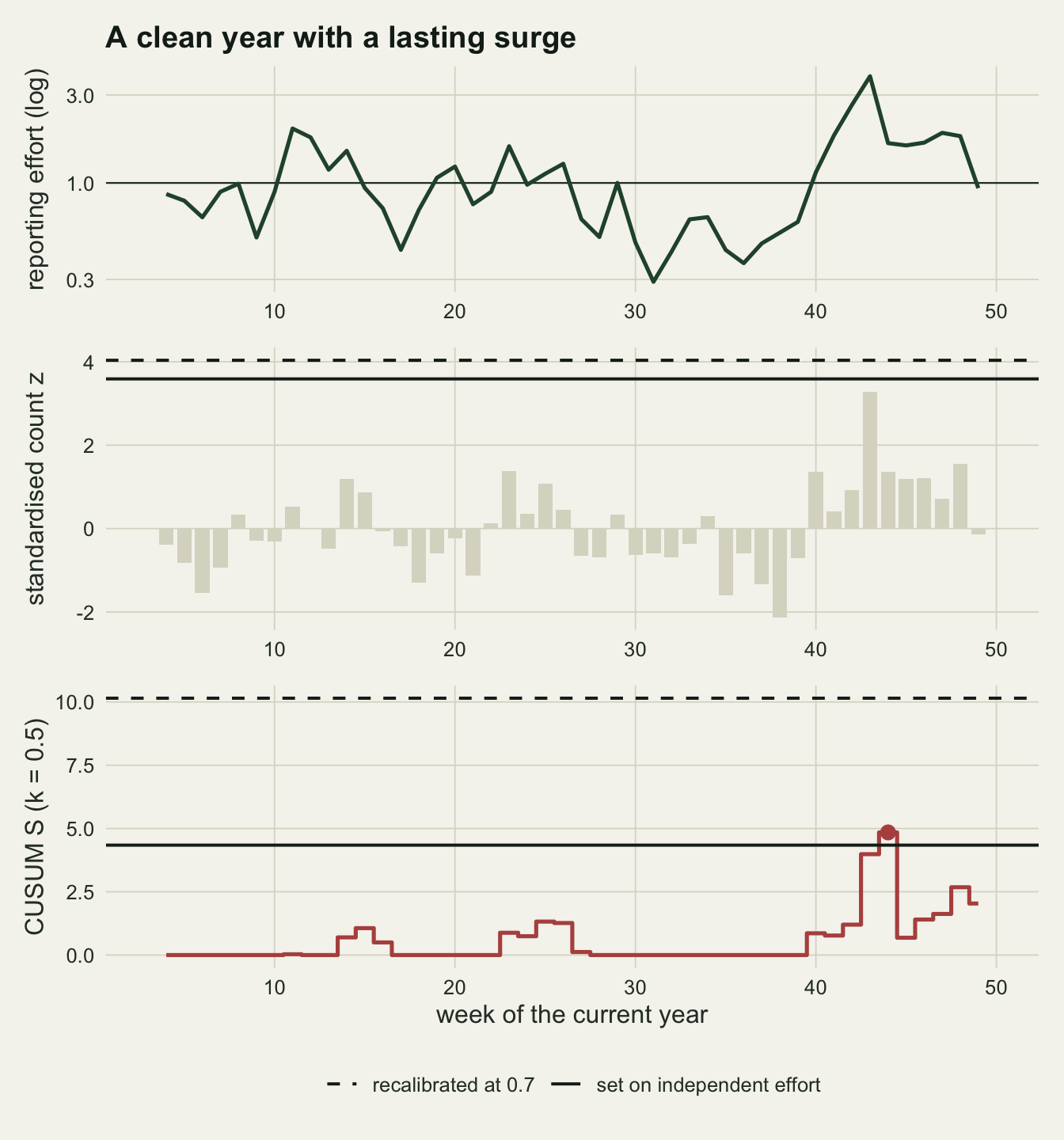
The figure shows the difference between the two rules in a year with nothing to find. Of the 4000 clean years of the sweep at an autocorrelation of 0.7, 53.8 per cent carry at least one alarm from the CUSUM with k = 0.5 at its threshold set on independent effort, and 23.7 per cent at least one from the single-week rule; in 30.8 per cent only the CUSUM alarms, and in 0.7 per cent only the single-week rule. The year drawn is the first CUSUM-only year among 200 years simulated for the figure. Reporting effort stays above its average for 9 weeks in a row, from week 40 to week 48. The standardised count is positive in 9 of those weeks and never higher than 3.28, below both single-week thresholds, but the CUSUM adds the weeks up and crosses its threshold in week 44. The threshold that holds the same CUSUM at 0.23 false alarms a year under this autocorrelation (dashed) is 10.15, against 4.34. The next sections measure what each of those two positions costs.
On independent effort the CUSUM earns its place over four weeks
With independent weekly effort, the setting of the source post, the three rules at 0.23 false alarms a year detect a 25-carcass die-off over two weeks with probability 0.321 (single week), 0.349 (CUSUM, k = 0.5) and 0.371 (CUSUM, k = 1). The source post’s guess holds here: the CUSUMs are ahead, by 0.029 and 0.051, both many standard errors from zero, though the gain is a few points of detection rather than a different class of rule.
Spread over four weeks, the same 25 carcasses (6.25 a week) are harder for every rule to see, and there the accumulation pays: the single-week rule detects 0.239, the CUSUMs 0.329 and 0.308. That is the case a CUSUM is built for, an excess too small to cross a single-week limit that lasts long enough to add up, and the smaller reference value, tuned for the smaller weekly shift, does better on it.
A CUSUM that is still climbing when the die-off ends may alarm a week later, which a scheme would still count as a find. Counting an alarm in the week after a two-week die-off as a detection raises the three figures only to 0.325, 0.375 and 0.387, so the definition of detection used here does not hide a large CUSUM advantage.
A reporting surge that lasts
fa_plot <- fa_tab
fa_plot$rule <- factor(fa_plot$rule, levels = rule_names)
ggplot(fa_plot, aes(rho, fa_fixed, colour = rule)) +
  geom_hline(yintercept = fa_target, linetype = "dashed", colour = te_body, linewidth = 0.6) +
  geom_errorbar(aes(ymin = fa_fixed - 2 * fa_fixed_se, ymax = fa_fixed + 2 * fa_fixed_se),
                width = 0.015, linewidth = 0.5) +
  geom_line(linewidth = 0.9) +
  geom_point(size = 2.2) +
  scale_colour_manual(values = rule_cols, name = NULL) +
  scale_y_continuous(limits = c(0, NA)) +
  labs(x = "lag-one autocorrelation of log reporting effort",
       y = "false alarms per year",
       title = "A lasting surge is what a CUSUM accumulates",
       subtitle = "thresholds calibrated to 0.23 a year on independent effort; bars: 2 standard errors") +
  theme_datasheet() + theme(legend.position = "bottom")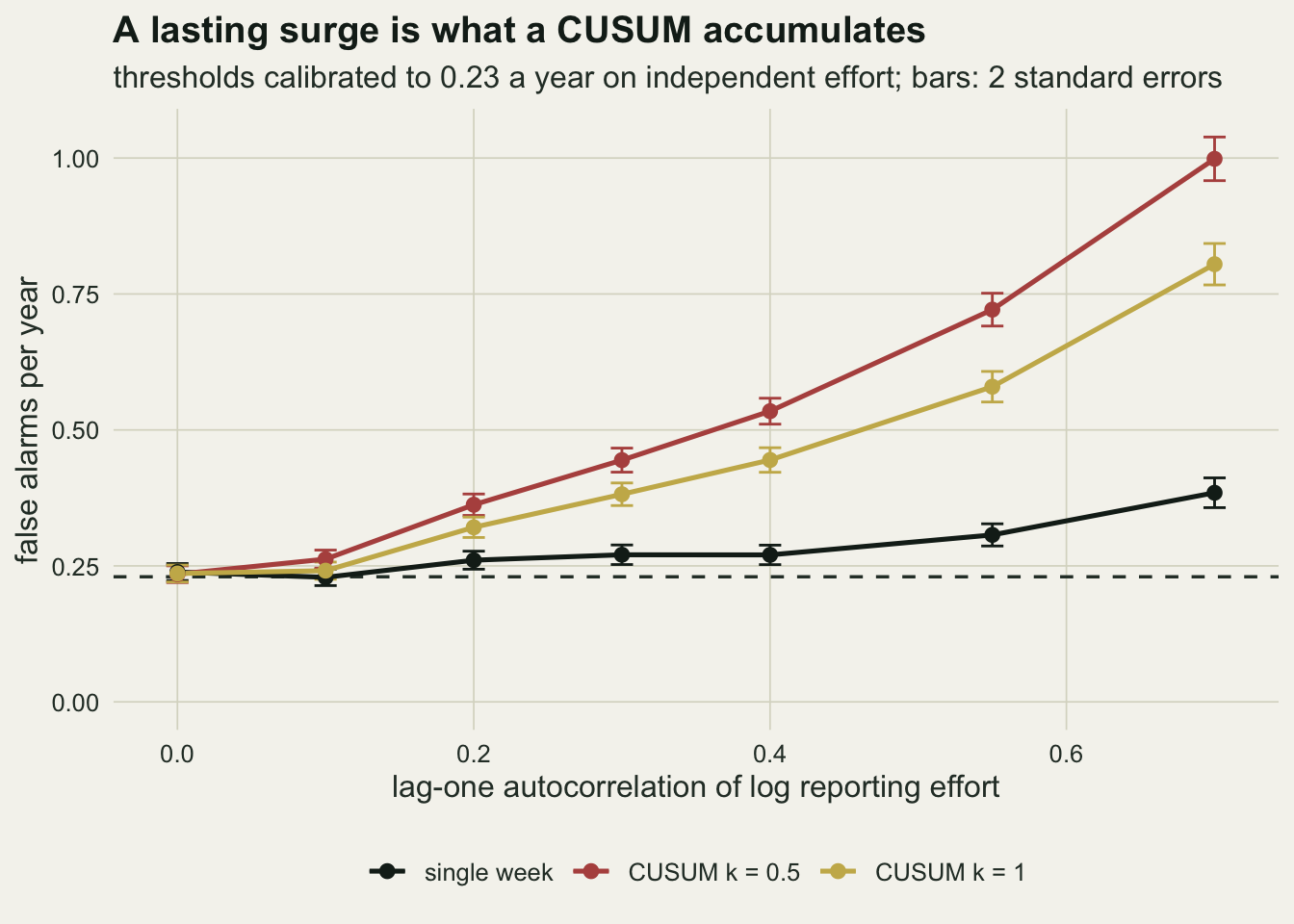
Now let reporting effort persist, and leave every threshold where the independent-effort calibration put it, as a scheme that never checked would. At an autocorrelation of 0.7 the single-week rule raises 0.385 false alarms a year, 1.6 times its rate on independent effort. The CUSUM with k = 0.5 raises 0.999, 4.3 times its own, and with k = 1 0.805. The CUSUM’s inflation starts early: at an autocorrelation of 0.2 the k = 0.5 scheme already runs at 0.362 a year, while the single-week rule is at 0.260.
This is the source post’s reporting surge read as a die-off, and the CUSUM is the rule most likely to read it that way. A news story that raises reports modestly for several weeks produces, week after week, exactly the small sustained excess that the CUSUM was designed to accumulate. The direction is what process control would predict; the size, on carcass counts with a thirty-five-week baseline, is the part a scheme needs.
At the same false alarm rate, the order reverses
first_behind <- function(dn, r) {
  d <- det_tab[det_tab$die_off == dn & det_tab$rule == r, ]
  below <- which(d$diff < -3 * d$diff_se)   # behind by more than three paired standard errors
  if (length(below) == 0) return(c(NA, NA))
  j <- min(below)
  c(if (j > 1) d$rho[j - 1] else NA, d$rho[j])
}
cross_f5 <- first_behind("fortnight", "CUSUM k = 0.5")
cross_f1 <- first_behind("fortnight", "CUSUM k = 1")
cross_4w5 <- first_behind("four weeks", "CUSUM k = 0.5")
cross_4w1 <- first_behind("four weeks", "CUSUM k = 1")
ratio_07 <- det_at(0.7, "fortnight", "CUSUM k = 0.5") / det_at(0.7, "fortnight", "single week")
ratio_07k1 <- det_at(0.7, "fortnight", "CUSUM k = 1") / det_at(0.7, "fortnight", "single week")
det_plot <- det_tab
det_plot$rule <- factor(det_plot$rule, levels = rule_names)
det_plot$die_off <- factor(det_plot$die_off, levels = c("fortnight", "four weeks"),
labels = c("25 carcasses over two weeks", "25 carcasses over four weeks"))
p_matched <- ggplot(det_plot, aes(rho, det, colour = rule, fill = rule)) +
geom_ribbon(aes(ymin = det - 2 * det_se, ymax = det + 2 * det_se), colour = NA, alpha = 0.25) +
geom_line(linewidth = 0.9) +
geom_point(size = 2) +
facet_wrap(~ die_off) +
scale_colour_manual(values = rule_cols, name = NULL) +
scale_fill_manual(values = rule_cols, name = NULL) +
scale_y_continuous(limits = c(0, NA)) +
labs(x = "lag-one autocorrelation of log reporting effort",
y = "probability of detection",
title = "Matched at 0.23 false alarms a year",
subtitle = "every threshold recalibrated under its own autocorrelation") +
theme_datasheet() +
theme(legend.position = "bottom", strip.text = element_text(colour = te_ink, face = "bold"))
p_matched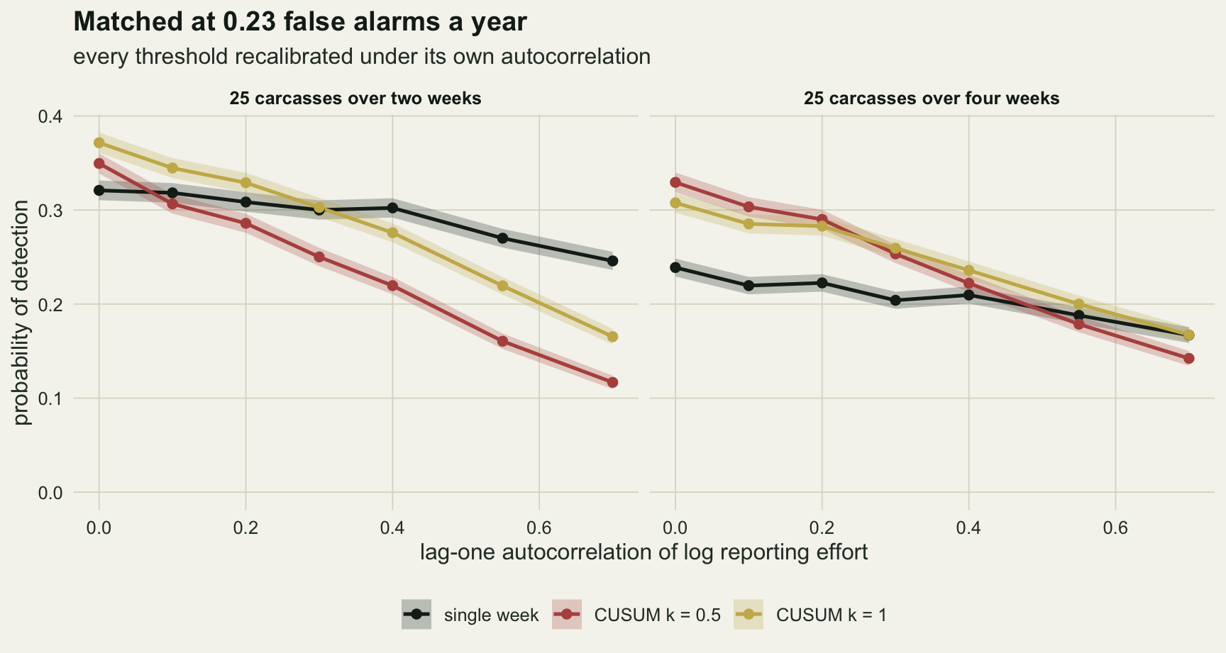
The fair comparison recalibrates every threshold under the autocorrelation the scheme has, so that all three rules again raise 0.23 false alarms a year, and then asks which detects more. At an autocorrelation of 0.4 the two-week die-off is detected with probability 0.302 by the single-week rule, 0.220 by the CUSUM with k = 0.5 and 0.276 with k = 1. At 0.7 the three figures are 0.246, 0.117 and 0.165: the CUSUM with k = 0.5 detects 0.47 times as often as the single-week rule, and with k = 1 0.67 times as often. The ordering the source post hinted at is reversed for both reference values.
How much the CUSUM loses depends on k. On independent effort the two-week die-off raises \(z\) by 2.20 on average in each of its weeks, where a clean week’s \(z\) has a standard deviation of 1.04, so a CUSUM tuned for this die-off would have k near 1.1, closer to 1 than to 0.5. A CUSUM with a larger k accumulates less and alarms more on single weeks, and as k grows it turns into a single-week rule. The factor of 0.47 belongs to the textbook k = 0.5; the better-tuned k = 1 loses less.
# the crossing for k = 0.5: redraw calibration years and die-offs four times
set.seed(33040)
rd_rho <- c(0.1, 0.2)
redraw <- do.call(rbind, lapply(rd_rho, function(rh) do.call(rbind, lapply(1:4, function(i) {
  cal <- run_years(n_cal, rh)$z
  th  <- sapply(rule_names[1:2], calibrate, z = cal)
  d   <- run_years(n_die, rh, D_size, 2)
  hr  <- sapply(rule_names[1:2], function(r) hits(alarms(d$z, r, th[[r]]), d$onset, 2))
  data.frame(rho = rh, rep = i, gap = mean(hr[, 2] - hr[, 1]),
             gap_se = sd(hr[, 2] - hr[, 1]) / sqrt(n_die))
}))))
rd <- function(rh, f) f(redraw$gap[redraw$rho == rh])
The reversal does not need strong persistence. For the two-week die-off the sweep puts the CUSUM with k = 0.5 behind the single-week rule already at an autocorrelation of 0.1, by 0.012 with a paired standard error of 0.004. That is one draw. Four fresh draws of the calibration years and the die-offs (the chunk above) give smaller gaps, from -0.009 to -0.004 with a mean of -0.006: at 0.1 the CUSUM is at most slightly behind. From 0.2 the CUSUM is clearly behind: by 0.023 in the sweep and by 0.021 to 0.032 in the redraws. The larger reference value keeps the CUSUM ahead for longer: at 0.3 it is level with the single-week rule (a difference of 0.003, standard error 0.003), and from 0.4 on it is behind. Moving k from 0.5 to 1 narrows the gap at high persistence but does not close it.
Over four weeks the CUSUMs hold their advantage much longer. With k = 0.5 the CUSUM is still slightly ahead at 0.4 (0.222 against 0.210, a paired standard error of 0.004), about level at 0.55 (a difference of -0.009) and behind more than three standard errors only at 0.7; with k = 1 it is ahead up to 0.55 and level at 0.7 (0.167 against 0.167). Every rule loses detection as the persistence grows, because every threshold has to rise, but the single-week rule loses least: its two-week detection falls from 0.321 to 0.246 between the two ends of the grid, the k = 0.5 CUSUM’s from 0.349 to 0.117.
Why the single-week limit moves at all
phi_df <- rbind(data.frame(rho = "independent effort", phi = sweep[[1]]$phi),
                data.frame(rho = "autocorrelation 0.7", phi = sweep[[length(sweep)]]$phi))
thr_rel <- do.call(rbind, lapply(rule_names, function(r) {
  d <- fa_tab[fa_tab$rule == r, ]
  data.frame(rho = d$rho, rule = r, rel = d$thr / d$thr[d$rho == 0])
}))
rel_07 <- setNames(thr_rel$rel[thr_rel$rho == 0.7], thr_rel$rule[thr_rel$rho == 0.7])
pw_back <- sapply(c("CUSUM k = 0.5", "CUSUM k = 1"), function(r)
  (det_at(0.7, "fortnight", r, "det_pw") - det_at(0.7, "fortnight", r)) /
    (det_at(0, "fortnight", r) - det_at(0.7, "fortnight", r)))
# prewhitened CUSUMs against the prewhitened single-week rule, four-week die-off
pw4 <- det_tab[det_tab$die_off == "four weeks" & det_tab$rule != "single week", ]
pw4_j <- which.min(pw4$diff_pp)
pw4_margin <- pw4$diff_pp[pw4_j]
pw4_margin_se <- pw4$diff_pp_se[pw4_j]
pw4_where <- pw4$rho[pw4_j]
pw4_rule <- pw4$rule[pw4_j]
pw4_z_min <- min(pw4$diff_pp / pw4$diff_pp_se)
# the single-week rule on prewhitened counts, two-week die-off
sw_pw <- det_tab[det_tab$die_off == "fortnight" & det_tab$rule == "single week", ]
sw_pw_low <- range(sw_pw$diff_pw[sw_pw$rho <= 0.4])
best07 <- det_tab[det_tab$rho == 0.7 & det_tab$die_off == "fortnight", ]
best07 <- max(c(best07$det, best07$det_pw))
The two rules need very different repairs. To hold 0.23 false alarms a year at an autocorrelation of 0.7, the single-week threshold rises by a factor of 1.12, the CUSUM thresholds by 2.34 (k = 0.5) and 2.15 (k = 1). A two-week die-off of 25 carcasses rarely climbs a CUSUM threshold raised that far, and that is the reversal.
For the CUSUM the cause is the one process control knows: its input now comes in runs. The lag-one autocorrelation of the standardised count in clean years is 0.15 at a log-effort autocorrelation of 0.2, 0.29 at 0.4 and 0.50 at 0.7, and it is the number a scheme can measure from its own counts. A sum of positively correlated terms spreads more widely than a sum of independent ones, so the same CUSUM threshold is crossed more often. For the raw counts this autocorrelation has a closed form. The effort’s own lag-one autocorrelation is \((e^{s^2\rho} - 1)/(e^{s^2} - 1)\); the effort multiplies the mean \(\mu\), so neighbouring counts have a covariance of \(\mu^2(e^{s^2\rho} - 1)\) and a variance of \(\mu + \mu^2(e^{s^2} - 1)\), because the Poisson draw adds a variance of \(\mu\) to each count without adding any covariance between weeks, so
\[r_y = \frac{\mu\,(e^{s^2\rho} - 1)}{1 + \mu\,(e^{s^2} - 1)}.\]
With \(\mu = 6\) and \(s = 0.6\) this gives 0.124, 0.258 and 0.478 at the same three values of \(\rho\). The standardised count computed with the true mean and dispersion follows it closely (0.131, 0.259 and 0.470 in the sweep). The small excess of the measured values comes from the baseline, 0.023 already on independent effort: neighbouring tested weeks share six of their seven baseline weeks in every year, so their baseline means move together.
For the single-week rule the runs in the current year are not the cause, because each week is compared with the limit once, whatever its neighbours did. The cause is the baseline. The dispersion is estimated from five blocks of seven consecutive weeks, and consecutive weeks under persistent effort are more alike than weeks in general, so the spread within a block understates the spread of a week. The median estimated dispersion falls from 3.21 on independent effort to 2.87 at 0.7, against a true 3.60, and the share of baselines below the truth rises from 63 to 71 per cent. Putting the true dispersion in place of the estimate, at the threshold calibrated on independent effort, gives 0.124 false alarms a year on independent effort and 0.139 at 0.7, a rise of 0.015 against the rise of 0.146 with the estimated dispersion. The single-week rule over-alarms under persistence almost entirely through the dispersion of its baseline.
thr_rel$rule <- factor(thr_rel$rule, levels = rule_names)
p_rel <- ggplot(thr_rel, aes(rho, rel, colour = rule)) +
  geom_hline(yintercept = 1, colour = te_body, linewidth = 0.4) +
  geom_line(linewidth = 0.9) + geom_point(size = 2) +
  scale_colour_manual(values = rule_cols, name = NULL) +
  labs(x = "autocorrelation of log effort", y = "threshold relative to independent effort",
       title = "What each rule must give up") +
  theme_datasheet() + theme(legend.position = "bottom")
phi_df$rho <- factor(phi_df$rho, levels = c("independent effort", "autocorrelation 0.7"))
p_phi <- ggplot(phi_df[phi_df$phi < 10, ], aes(phi, colour = rho)) +
  geom_density(linewidth = 0.9, adjust = 0.8, key_glyph = "path") +
  geom_vline(xintercept = phi_true, linetype = "dashed", colour = te_body, linewidth = 0.6) +
  scale_colour_manual(values = c(te_forest, te_rust), name = NULL) +
  labs(x = "estimated dispersion, 35 weeks", y = "density",
       title = "Correlated weeks look too alike") +
  theme_datasheet() + theme(legend.position = "bottom")
p_rel + p_phi + plot_annotation(theme = theme_datasheet())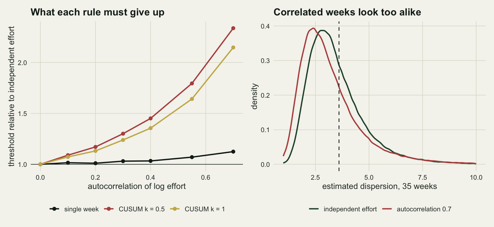
Prewhitening the standardised count
Alwan and Roberts’ repair for autocorrelated process data is to chart the residuals of a time series model instead of the raw observations. The simplest version filters the standardised count with its own lag-one autocorrelation \(r\),
\[u_t = \frac{z_t - r\,z_{t-1}}{\sqrt{1 - r^2}},\]
and runs every rule on \(u\), recalibrated to 0.23 false alarms a year. Here \(r\) is estimated from the clean calibration years, which stands in for a scheme estimating it from its own past residuals. The filter has a price in the second week of a die-off, because it subtracts \(r\) times a previous week whose count already carries the die-off.
At an autocorrelation of 0.7, prewhitening raises the two-week detection of the CUSUM from 0.117 to 0.213 with k = 0.5 and from 0.165 to 0.269 with k = 1, and that of the single-week rule from 0.246 to 0.290. The prewhitened CUSUM with k = 1 now detects 0.023 more than the plain single-week rule (standard error 0.002), but the single-week rule gains from the same filter and stays ahead of it. Over four weeks the prewhitened CUSUMs are ahead again, the k = 1 scheme clearly: 0.182 and 0.191 against 0.173 for the prewhitened single-week rule (paired standard errors 0.004 and 0.003). At 0.4 the filter changes the single-week rule little (0.302 to 0.299 over two weeks) and brings the k = 1 CUSUM to 0.308, about level with the plain single-week rule: 0.006 above it, with a paired standard error of 0.003 that does not count the error in the two thresholds.
Prewhitening wins back 42 and 50 per cent of what the two CUSUMs lost between independent effort and 0.7 over two weeks, but neither catches up with the prewhitened single-week rule. For the die-off spread over four weeks, both prewhitened CUSUMs detect more than the prewhitened single-week rule at every persistence on the grid. The smallest margin is 0.009, for the CUSUM with k = 0.5 at 0.7, 2.3 times its paired standard error of 0.004; there the two are close to level once threshold error is allowed for.
pw_df <- det_tab[det_tab$rho %in% c(0.4, 0.7), ]
pw_long <- rbind(data.frame(pw_df[, c("rho", "die_off", "rule")], input = "raw z", det = pw_df$det),
                 data.frame(pw_df[, c("rho", "die_off", "rule")], input = "prewhitened z", det = pw_df$det_pw))
pw_long$input <- factor(pw_long$input, levels = c("raw z", "prewhitened z"))
pw_long$panel <- paste0("autocorrelation ", pw_long$rho)
pw_long$die_off <- factor(pw_long$die_off, levels = c("fortnight", "four weeks"),
                          labels = c("over two weeks", "over four weeks"))
ggplot(pw_long, aes(det, rule, colour = input, shape = input)) +
  geom_line(aes(group = rule), colour = te_line, linewidth = 1) +
  geom_point(size = 3) +
  facet_grid(die_off ~ panel) +
  scale_colour_manual(values = c(te_rust, te_forest), name = NULL) +
  scale_shape_manual(values = c(16, 17), name = NULL) +
  scale_y_discrete(limits = rev(rule_names)) +
  labs(x = "probability of detection at 0.23 false alarms a year", y = NULL,
       title = "Prewhitening helps the CUSUMs most") +
  theme_datasheet() +
  theme(legend.position = "bottom", strip.text = element_text(colour = te_ink, face = "bold"))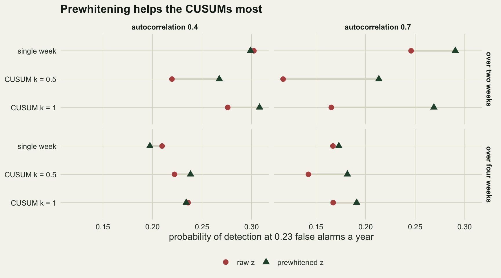
What to report
Report the false alarm rate each rule runs at under the scheme’s own week-to-week persistence, measured on simulated clean years that carry that persistence. A threshold calibrated on independent weeks is not a statement about a scheme whose reporting effort persists: at a log-effort autocorrelation of 0.7, the CUSUM with k = 0.5 set that way ran at 0.999 false alarms a year against its target of 0.23.
Measure the persistence. The lag-one autocorrelation of the standardised counts in weeks without a known die-off is the observable quantity. In this simulation the plain CUSUM with k = 0.5 fell clearly behind the single-week rule for a two-week die-off somewhere between a measured value of 0.09 (log-effort autocorrelation 0.1) and 0.15 (0.2), and the k = 1 scheme between 0.22 and 0.29. A scheme with five years of history has about 230 tested weeks to estimate it from, and in the sweep the value estimated from five clean years scatters with a standard deviation of 0.075 at 0.2: wider than either crossing interval, so a scheme cannot tell from its own counts which side of the crossing it is on.
Compare rules at a matched false alarm rate, and for a stated die-off. Which rule is better depends on how the die-off is spread: here, once the log-effort autocorrelation reached 0.4, the single-week limit detected 25 carcasses in two weeks more often than either plain CUSUM, while for 25 carcasses in four weeks the CUSUM with k = 1 stayed ahead or level at every persistence on the grid. State the reference value k with any CUSUM: which of the two values did better depended here on both the duration of the die-off and the persistence. At 0.7 the best rule for the two-week die-off was not a CUSUM at all but the single-week rule on prewhitened counts, at 0.290.
State the share of years with at least one false alarm as well, as the source post asks, because matching on alarm weeks does not match it. At 0.7 and at matched thresholds, the single-week rule raises at least one false alarm in 0.163 of clean years, the CUSUM in 0.189 (k = 0.5) and 0.181 (k = 1): the single-week rule’s false alarms come more often several to a year. Matched on the share of disturbed years instead, its threshold could come down and its detection go up, so the comparison here, if anything, favours the CUSUM.
If a CUSUM is run where reporting effort persists, run it on prewhitened counts and recalibrate it there, and report the autocorrelation used for the filter. The single-week rule gains from the same filter at strong persistence (0.246 to 0.290 at 0.7), but not at 0.4 or below, where it changed the two-week detection by -0.011 to -0.003.
Honest limits
The simulation is the source post’s flat control: a mean of six a week, reporting noise with log-scale standard deviation 0.6, one die-off size and two durations. The persistence is an AR(1) process on log effort. A news story is closer to a step that decays than to a stationary AR(1), and a scheme’s persistence may change with the season; neither was simulated, and the source post’s seasonal arms were not rerun with a CUSUM.
The recalibration uses the true autocorrelation and 16000 simulated clean years for each threshold, and the prewhitening filter uses a lag-one autocorrelation estimated from those same clean years. A scheme has a few years of its own history, containing its own past die-offs, to estimate both from; the extra error that brings to the false alarm rate was not measured. The comparison at matched rates is the comparison of rules, not of what a particular scheme would achieve with its estimated thresholds.
Only the simplest one-sided CUSUM of Page on Farrington’s standardised count was run, with two reference values and a reset to zero after each alarm. The two-week die-off would call for a k near 1.1, and larger values were not run; since a CUSUM with a large k approaches the single-week rule, the size of the CUSUM’s loss depends on k, and the loss quoted for k = 0.5 is the larger of the two measured. Variants with a head start after an alarm, CUSUMs on a negative binomial likelihood ratio, and the CUSUM methods in the surveillance package were not tried. Prewhitening with one lag coefficient is the simplest residual chart; a count model with a lag term, fitted to the scheme’s history, might keep more of the CUSUM’s multi-week advantage, and it was not tried either.
Detection is counted in the die-off’s own weeks, with a one-week grace period checked once. How soon after onset each rule alarms, and how the answer changes when a die-off itself draws publicity and more reporting (the second limit of the source post), were not measured.
References
Alwan LC, Roberts HV 1988 Journal of Business and Economic Statistics 6(1):87-95 (10.1080/07350015.1988.10509640)
Farrington CP, Andrews NJ, Beale AD, Catchpole MA 1996 Journal of the Royal Statistical Society Series A 159(3):547-563 (10.2307/2983331)
Lu C-W, Reynolds MR 2001 Journal of Quality Technology 33(3):316-334 (10.1080/00224065.2001.11980082)
Page ES 1954 Biometrika 41(1-2):100-115 (10.1093/biomet/41.1-2.100)
Unkel S, Farrington CP, Garthwaite PH, Robertson C, Andrews N 2012 Journal of the Royal Statistical Society Series A 175(1):49-82 (10.1111/j.1467-985X.2011.00714.x)