library(ggplot2)

te_paper  <- "#f5f4ee"
te_ink    <- "#16241d"
te_body   <- "#2c3a31"
te_forest <- "#275139"
te_rust   <- "#b5534e"
te_gold   <- "#c9b458"
te_line   <- "#dad9ca"

theme_datasheet <- function() {
  theme_minimal(base_size = 12) +
    theme(plot.background  = element_rect(fill = te_paper, colour = NA),
          panel.background = element_rect(fill = te_paper, colour = NA),
          panel.grid.major = element_line(colour = te_line, linewidth = 0.3),
          panel.grid.minor = element_blank(),
          text             = element_text(colour = te_body),
          plot.title       = element_text(colour = te_ink, face = "bold"),
          plot.subtitle    = element_text(colour = te_body),
          axis.text        = element_text(colour = te_body),
          strip.text       = element_text(colour = te_ink))
}Chilling, forcing and projected leaf-out
R
phenology
climate change
simulation
ecology tutorial
A forcing-only degree day model of spring leaf-out misstates the advance under warming, and gets its sign wrong where winter chill runs out. Measured in R.
A forest reserve has forty years of leaf-out dates for a beech stand and a weather station a kilometre away. The obvious model is thermal time: add up degree days from some date in winter and call leaf-out the day the sum reaches a fixed requirement. It is fitted to the forty years, and the next step is to run it on a climate four degrees warmer and report how many days earlier the leaves will come.
Many temperate trees do not work that way. Their buds need a spell of winter cold before spring warmth has its full effect, and the more cold they have had, the less warmth they need. The classic form of this idea, from Cannell and Smith (1983), makes the forcing requirement a negative exponential function of the number of chill days, with chilling and forcing accumulating side by side; it is known in phenology modelling as the alternating model, and Chuine (2000) showed that the widely used budburst models are particular cases of one general model. Under this model warming does two things at once. It adds forcing, which brings leaf-out earlier, and it removes chill, which raises the requirement and pushes leaf-out later. A forcing-only model sees the first and not the second.
This site already has one post with the same structure. The section “What thermal time cannot do” in Degree days and thermal time in R calibrates a linear degree day model on twenty baseline years and shows it predicting the completion of a late-summer development stage too early in a year five degrees hotter, because the true development rate is a curve that bends down past its optimum. That is the forcing-shape sibling of this post: there the rate curve is wrong, here the rate is exactly linear and the requirement itself moves. Phenological trends and temperature estimates the usual days-per-degree sensitivity and shows how rising observer effort in warm years inflates the first-date version of it; the regression below uses the mean date, has no effort problem, and fails for a different reason, which is extrapolation. Climate window analysis in R finds the stretch of the calendar whose weather best predicts a response and ends by warning that a window is not a mechanism. A projection needs the mechanism, and here it is known by construction.
The result is not new to tree phenology. That warming can delay budburst where winters become too mild to chill the buds is a long-standing expectation of chilling models, and Fu and colleagues (2015) reported that the apparent advance of spring leaf unfolding per degree of warming in European trees has declined, with reduced winter chilling proposed as part of the cause. Gao and colleagues (2024) argue that chilling effects estimated from field records are partly statistical artefacts and that the loss of chill may not limit near-future advances much. This post does not settle that argument; its tree has a chilling requirement by construction. It demonstrates what the usual tools do to a projection when chilling matters, how much of that can be seen in the fitting years, and what happens when the chilling model itself is fitted with the wrong chill rule.
A tree that needs winter before spring
The simulated year runs from 1 September, so day 62 is 1 November and day 123 is 1 January. Daily mean temperature is a seasonal cosine with its minimum in mid January and a half range of 8 degrees, plus a whole-year anomaly (SD 1.2), a separate spring anomaly from 1 January (SD 1), and day-to-day noise that follows a first-order autoregression with coefficient 0.75. The spring anomaly lets a cold winter be followed by a warm spring, so that chill and forcing are not locked together from year to year.
The tree follows the alternating model. A chill day is a day whose mean is below 5 C, counted from 1 November. Forcing is the sum of degree days above 5 C from 1 January (Cannell and Smith counted forcing from 1 February; the earlier start here is this post’s choice). Leaf-out is the first day on which the forcing sum reaches a + b exp(-c C), where C is the number of chill days so far; both sums keep running until that day. The constants a = 40, b = 700 and c = 0.03 are this post’s choices, not estimates for any species, and the thresholds and start dates are fixed design constants.
n_day <- 365; day <- seq_len(n_day)           # day 1 = 1 September
chill_start <- 62; force_start <- 123         # 1 November, 1 January
t_chill <- 5; t_base <- 5                     # chill: mean below 5 C; forcing: above 5 C
a_true <- 40; b_true <- 700; c_true <- 0.03   # requirement a + b exp(-c C)
amp <- 8; feb1 <- 154; apr30 <- 242           # half the seasonal range; 1 Feb, 30 Apr

clim_of     <- function(t_ann) t_ann - amp * cos(2 * pi * (day - 137) / 365)
winter_mean <- function(t_ann) mean(clim_of(t_ann)[chill_start:(force_start + 58)])

weather_anom <- function(n_yr, burn = 60) {
  e_mat  <- matrix(rnorm((n_day + burn) * n_yr, 0, 1.8), ncol = n_yr)
  ar_mat <- stats::filter(e_mat, 0.75, method = "recursive")
  ar_mat <- t(ar_mat[-seq_len(burn), , drop = FALSE])
  ar_mat + rnorm(n_yr, 0, 1.2) + outer(rnorm(n_yr, 0, 1), as.numeric(day >= force_start))
}

row_cumsum <- function(m) t(apply(m, 1, cumsum))
chill_days <- function(temp, rule = list(lo = -Inf, hi = t_chill, start = chill_start))
  row_cumsum((temp >= rule$lo & temp < rule$hi) * rep(day >= rule$start, each = nrow(temp)))
forcing <- function(temp, base = t_base, start = force_start)
  row_cumsum(pmax(temp - base, 0) * rep(day >= start, each = nrow(temp)))
first_day  <- function(h, thr) pmin(rowSums(h < thr) + 1, n_day)
first_days <- function(h, thr)
  pmin(t(vapply(seq_len(nrow(h)), function(i) findInterval(thr, h[i, ], left.open = TRUE) + 1,
                numeric(length(thr)))), n_day)
leaf_out <- function(temp)
  first_day(forcing(temp) - b_true * exp(-c_true * chill_days(temp)), a_true)
chill_at_leaf <- function(temp) {
  lo <- leaf_out(temp)
  chill_days(temp)[cbind(seq_along(lo), lo)]
}

set.seed(4317)
check_temp <- weather_anom(30) + rep(clim_of(10), each = 30)
h_check <- forcing(check_temp) - b_true * exp(-c_true * chill_days(check_temp))
stopifnot(all(apply(h_check, 1, diff) >= 0))
slow_check <- sapply(seq_len(30), function(i) {
  frc <- cumsum(pmax(check_temp[i, ] - t_base, 0) * (day >= force_start))
  chl <- cumsum((check_temp[i, ] < t_chill) * (day >= chill_start))
  which(frc >= a_true + b_true * exp(-c_true * chl))[1]
})
stopifnot(identical(as.numeric(leaf_out(check_temp)), as.numeric(slow_check)))
The vectorised leaf-out rule counts the days on which forcing minus b exp(-c C) is still below a. That is only the first crossing if the difference never falls, and the first stopifnot line checks that it does not: forcing only grows and the chill term only shrinks. The second compares the vectorised rule with a plain day-by-day search on thirty years and finds the same dates. Two limits follow from the formula. With unlimited chill the requirement falls to a, and with no chill at all it rises to a + b, 740 degree days; in both limits the tree is a forcing-only tree with a fixed requirement. Everything below happens between them.
Nine sites along a winter gradient
The same tree grows at nine sites that differ only in their mean temperature, with annual means from 5 to 15 C. The axis used throughout is the site’s mean temperature from November to February. Every site sees the same weather anomalies, so the sweep is smooth, and warming is a uniform shift of every day by 2 or 4 degrees. The true change in mean leaf-out date comes from the same 200 simulated years run in the present climate and in the warmer one.
t_ann_set <- seq(5, 15, by = 1.25); warm_set <- c(2, 4); n_proj <- 200
site_tab  <- data.frame(site = seq_along(t_ann_set), t_ann = t_ann_set,
                        winter = sapply(t_ann_set, winter_mean))

set.seed(4318)
anom_proj <- weather_anom(n_proj)
mech <- do.call(rbind, lapply(site_tab$site, function(s) {
  t_now <- anom_proj + rep(clim_of(site_tab$t_ann[s]), each = n_proj)
  do.call(rbind, lapply(c(0, warm_set), function(w) {
    temp  <- t_now + w
    lo    <- leaf_out(temp)
    ch_lo <- chill_at_leaf(temp)
    data.frame(site = s, winter = site_tab$winter[s], warm = w, leaf = mean(lo),
               chill = mean(ch_lo), need = mean(a_true + b_true * exp(-c_true * ch_lo)),
               chill_min = min(ch_lo), capped = sum(lo >= n_day))
  }))
}))
stopifnot(all(mech$capped == 0))
mech$shift <- mech$leaf - rep(mech$leaf[mech$warm == 0], each = 1 + length(warm_set))
m4 <- mech[mech$warm == 4, ]; m0 <- mech[mech$warm == 0, ]; m2 <- mech[mech$warm == 2, ]
doy_now <- m0$leaf - (force_start - 1)

set.seed(4320)
seed_shift <- sapply(1:8, function(k) {
  anom_k <- weather_anom(n_proj)
  sapply(site_tab$site, function(s) {
    t_now <- anom_k + rep(clim_of(site_tab$t_ann[s]), each = n_proj)
    mean(leaf_out(t_now + 4)) - mean(leaf_out(t_now))
  })
})
delay_sites <- which(m4$shift > 0)
delay2      <- which(m2$shift > 0)
seed_range  <- apply(seed_shift, 1, range)
stopifnot(all(seed_shift[delay_sites, ] > 0), length(delay_sites) == 3,
          all(diff(delay_sites) == 1), all(diff(delay2) == 1))
The November to February means run from -1.4 to 8.6 C. In the present climate the mean leaf-out date falls between day 96 and day 124 of the calendar year at every site, early April to early May. What changes along the gradient is how the tree gets there. At the coldest site it has collected 160 chill days by leaf-out and needs only 47 degree days of forcing; at the mildest it has 19 chill days and needs 472.
chill_panels <- c("chill days by leaf-out", "forcing requirement at leaf-out (degree days)")
chill_long <- data.frame(winter = mech$winter, value = c(mech$chill, mech$need),
  warm_lab = factor(mech$warm, c(0, 2, 4), c("present climate", "plus 2 C", "plus 4 C")),
  panel = factor(rep(chill_panels, each = nrow(mech)), chill_panels))
ggplot(chill_long, aes(winter, value, colour = warm_lab)) +
  geom_line(linewidth = 0.9) +
  geom_point(size = 2) +
  facet_wrap(~ panel, scales = "free_y") +
  scale_colour_manual(values = c(te_forest, te_gold, te_rust), name = NULL) +
  labs(x = "site mean temperature, November to February (C)", y = NULL,
       title = "Warming takes chill away and raises the requirement") +
  theme_datasheet() +
  theme(legend.position = "bottom")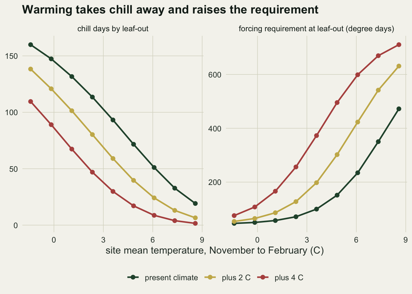
Four degrees of warming removes chill everywhere, because a chill day here is any day below 5 C and a warmer winter has fewer of them. The coldest site drops from 160 to 110 chill days, but it had so many that its requirement only moves from 47 to 76 degree days. At the site with a winter mean of 3.6 C the chill falls from 93 to 30 days and the requirement rises from 100 to 373. The mildest site already had little chill, and its requirement rises from 472 towards the ceiling of 740, reaching 711.
The true change in leaf-out date follows from that. At plus 4 C the tree comes out 24.0 days earlier at the coldest site, but at the three sites with winter means from 3.6 to 6.1 C it comes out later, by 3.8, 7.5 and 5.2 days: the added forcing does not pay for the added requirement. At the mildest site the requirement is already high in the present climate and can only rise to its ceiling, so the extra forcing wins again and leaf-out is 10.6 days earlier. At plus 2 C the delay appears at the sites with winter means from 4.8 to 7.3 C. The sign of the delay does not depend on the particular 200 years: over eight further independent sets of 200 years, the plus 4 C change at the three delay sites stays between 2.6 and 6.0, 6.4 and 8.7, and 4.6 and 5.8 days.
What an analyst would fit
Three models are fitted to each forty-year record, all by minimising the root mean square error (RMSE) of the predicted leaf-out day. The forcing-only model is the usual thermal time model with its three choices estimated: a base temperature from 0 to 8 C, a start date from 1 December to 1 April in steps of about a fortnight, and a requirement on a grid of 5 degree days. The days-per-degree model is a linear regression of leaf-out day on the mean temperature from February to April, and its projection is its slope times the warming, since a uniform shift raises that mean by exactly the warming. The chilling-forcing refit is the alternating model with the right chill rule, fitted over a grid of a, b and c that does not contain the true values (the stopifnot line checks that). Two more chilling-forcing fits, with a wrong chill rule, wait for a later section.
rmse <- function(p, y) sqrt(colMeans((p - y)^2))
fo_grid  <- expand.grid(base = 0:8,
                        start = c(92, 107, 123, 138, 154, 168, 182, 197, 213))
req_grid <- seq(5, 2000, by = 5)
fit_fo <- function(temp, y) {
  best <- list(rmse = Inf)
  for (i in seq_len(nrow(fo_grid))) {
    r <- rmse(first_days(forcing(temp, fo_grid$base[i], fo_grid$start[i]), req_grid), y)
    k <- which.min(r)
    if (r[k] < best$rmse) best <- list(rmse = r[k], base = fo_grid$base[i],
                                       start = fo_grid$start[i], req = req_grid[k])
  }
  best
}
pred_fo <- function(fit, temp) first_day(forcing(temp, fit$base, fit$start), fit$req)

rules <- list(known  = list(lo = -Inf, hi = 5, start = 62),
              window = list(lo = 0,    hi = 7, start = 62),
              late   = list(lo = -Inf, hi = 5, start = 92))
c_grid <- seq(0.0075, 0.0775, by = 0.005)
b_grid <- seq(150, 1950, by = 100)
a_grid <- seq(2.5, 297.5, by = 5)
stopifnot(!(c_true %in% c_grid), !(b_true %in% b_grid), !(a_true %in% a_grid))
fit_cf <- function(temp, y, rule, cg = c_grid, bg = b_grid, ag = a_grid) {
  chill <- chill_days(temp, rule)
  frc   <- forcing(temp)
  best  <- list(rmse = Inf)
  for (cc in cg) {
    e_chill <- exp(-cc * chill)
    for (bb in bg) {
      r <- rmse(first_days(frc - bb * e_chill, ag), y)
      k <- which.min(r)
      if (r[k] < best$rmse) best <- list(rmse = r[k], a = ag[k], b = bb, c = cc)
    }
  }
  best$rule <- rule
  best
}
pred_cf <- function(fit, temp)
  first_day(forcing(temp) - fit$b * exp(-fit$c * chill_days(temp, fit$rule)), fit$a)
spring_temp <- function(temp) rowMeans(temp[, feb1:apr30])
Each record is forty years of fresh weather at the site, with the true leaf-out day plus an observation error drawn with an SD of 3 days and rounded to a whole day. There are sixteen independent records per site. Each fitted model is then run on the same 200 present-climate years and on those years warmed, and its projected change is compared with the true one from the same years.
n_rep <- 16; n_fit <- 40; obs_sd <- 3
set.seed(4319)
mc <- list()
for (r in seq_len(n_rep)) {
  anom_fit <- weather_anom(n_fit)
  obs_err  <- round(rnorm(n_fit, 0, obs_sd))
  for (s in site_tab$site) {
    t_fit  <- anom_fit + rep(clim_of(site_tab$t_ann[s]), each = n_fit)
    y      <- leaf_out(t_fit) + obs_err
    fo     <- fit_fo(t_fit, y)
    cf     <- lapply(rules, function(rl) fit_cf(t_fit, y, rl))
    lm_fit <- lm(y ~ spring_temp(t_fit))
    t_now  <- anom_proj + rep(clim_of(site_tab$t_ann[s]), each = n_proj)
    for (w in warm_set) {
      t_w   <- t_now + w
      shift <- function(f) mean(f(t_w)) - mean(f(t_now))
      mc[[length(mc) + 1]] <- data.frame(rep = r, site = s, winter = site_tab$winter[s],
        warm = w, truth = mech$shift[mech$site == s & mech$warm == w],
        fo = shift(function(x) pred_fo(fo, x)),
        known = shift(function(x) pred_cf(cf$known, x)),
        window = shift(function(x) pred_cf(cf$window, x)),
        late = shift(function(x) pred_cf(cf$late, x)),
        lm = w * unname(coef(lm_fit)[2]),
        r_fo = fo$rmse, r_known = cf$known$rmse, r_window = cf$window$rmse,
        r_late = cf$late$rmse, r_lm = sqrt(mean(resid(lm_fit)^2)),
        fo_base = fo$base, fo_start = fo$start)
    }
  }
}
mc <- do.call(rbind, mc)
stopifnot(nrow(mc) == n_rep * nrow(site_tab) * length(warm_set))

cols <- c("truth", "fo", "known", "window", "late", "lm",
          "r_fo", "r_known", "r_window", "r_late", "r_lm")
agg <- aggregate(mc[, cols], by = list(warm = mc$warm, site = mc$site), FUN = mean)
agg$winter <- site_tab$winter[agg$site]
mse <- aggregate(mc[, c("fo", "known", "window", "late", "lm")],
                 by = list(warm = mc$warm, site = mc$site),
                 FUN = function(v) sd(v) / sqrt(length(v)))
se_max <- max(unlist(mse[, c("fo", "known", "lm")]))
a4 <- agg[agg$warm == 4, ]; a2 <- agg[agg$warm == 2, ]
gap4 <- a4$fo - a4$truth; gap2 <- a2$fo - a2$truth
worst <- which.max(abs(gap4)); worst2 <- which.max(abs(gap2))
lm_further <- sum(abs(a4$lm - a4$truth) > abs(gap4))
se_known4  <- max(mse$known[mse$warm == 4])
stopifnot(gap4[1] < 0, gap4[9] > 0, all(diff(abs(gap4[1:worst])) > 0),
          all(gap2 < 0), all(a2$fo[delay2] < 0),
          all(abs(a4$known - a4$truth) < 1.5 * mse$known[mse$warm == 4]))
Over the sixteen records the Monte Carlo standard error of a site’s mean projected change is at most 2.2 days for the forcing-only, days-per-degree and right-rule chilling-forcing fits.
Projected change across the sweep
band <- aggregate(known ~ warm + site, mc, range)
band <- data.frame(warm = band$warm, winter = site_tab$winter[band$site],
                   lo = band$known[, 1], hi = band$known[, 2])
sweep_long <- do.call(rbind, lapply(c("fo", "lm", "known", "truth"), function(v)
  data.frame(winter = agg$winter, warm = agg$warm, model = v, shift = agg[[v]])))
sweep_long$model <- factor(sweep_long$model, c("fo", "lm", "known", "truth"),
  c("forcing only", "days per degree", "chilling-forcing refit", "truth"))
panel_lab <- function(w) factor(sprintf("plus %d C", w), c("plus 2 C", "plus 4 C"))
sweep_long$panel <- panel_lab(sweep_long$warm)
band$panel <- panel_lab(band$warm)
sweep_plot <- function(dat, bnd) {
  ggplot(dat, aes(winter, shift)) +
    geom_hline(yintercept = 0, colour = te_body, linewidth = 0.4) +
    geom_ribbon(data = bnd, aes(winter, ymin = lo, ymax = hi), inherit.aes = FALSE,
                fill = te_forest, alpha = 0.15) +
    geom_line(aes(colour = model, linetype = model), linewidth = 0.9) +
    geom_point(aes(colour = model), size = 1.9) +
    facet_wrap(~ panel) +
    scale_colour_manual(values = c(te_rust, te_gold, te_forest, te_ink), name = NULL) +
    scale_linetype_manual(values = c("solid", "solid", "solid", "22"), name = NULL) +
    labs(x = "site mean temperature, November to February (C)",
         y = "change in mean leaf-out date (days)",
         title = "Forcing alone projects an advance where the tree is delayed") +
    theme_datasheet() +
    theme(legend.position = "bottom", legend.key.width = unit(1.6, "lines"))
}
sweep_plot(sweep_long, band)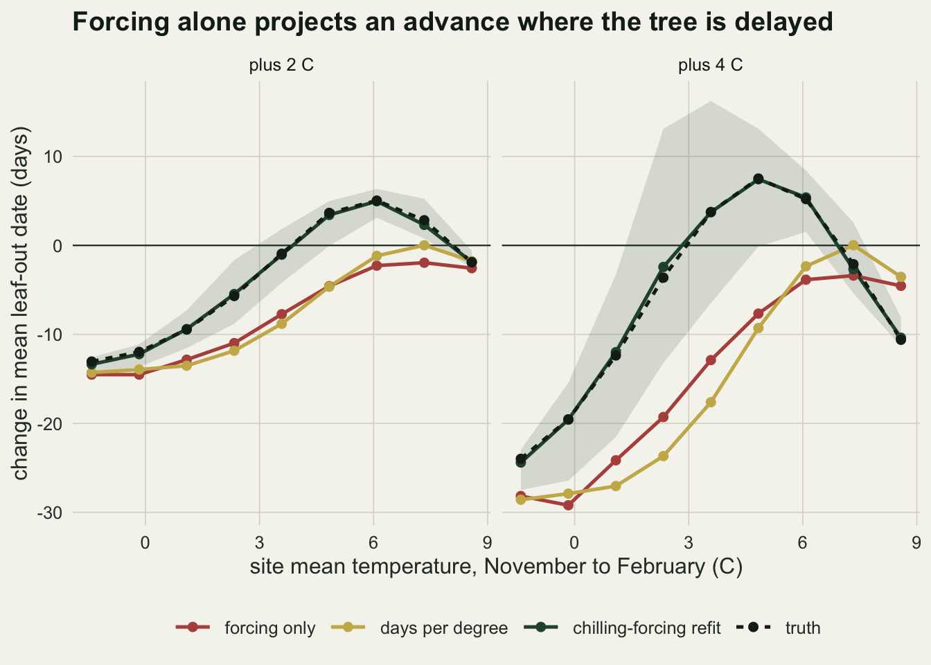
At plus 4 C and the coldest site the forcing-only model projects an advance of 28.2 days against a true 24.0, too much by 4.2 days. The gap widens towards milder winters, to a maximum of 16.6 days at the site with a winter mean of 3.6 C, and narrows beyond it. At the site with a winter mean of 1.1 C the projection is 24.2 days earlier where the truth is 12.4, 1.95 times the true advance, and at the three delay sites the forcing-only model projects advances of 12.9, 7.7 and 3.9 days where the tree is in fact later. At the mildest site the error changes sign: the forcing-only model projects only 4.5 days of advance against a true 10.6. There is no single overstatement factor; size and sign depend on where the site’s winter sits relative to the chill threshold.
The days-per-degree regression behaves much like the forcing-only model and is further from the truth than it at 7 of the nine sites: at the delay sites it projects 17.6, 9.3 and 2.3 days of advance. At plus 2 C the forcing-only model overstates the advance or misses the delay at every site, with no sign change at the mild end; its largest gap is 8.2 days, at the site with a winter mean of 4.8 C. The chilling-forcing refit with the right rule shows no bias beyond Monte Carlo error: its mean projection is within 1.2 days of the truth at every site at plus 4 C, against a Monte Carlo SE of up to 2.2 days. The shaded band is the other half of that story, and it is taken up below.
The past already separates the two models
The forcing-only model fits the forty years it was calibrated on less well than the chilling-forcing refit at every site, and much less well at the milder ones; that is visible without any projection.
rmse_long <- do.call(rbind, lapply(c("r_fo", "r_lm", "r_known"), function(v)
  data.frame(winter = a4$winter, model = v, rmse = a4[[v]])))
rmse_long$model <- factor(rmse_long$model, c("r_fo", "r_lm", "r_known"),
  c("forcing only", "days per degree", "chilling-forcing refit"))
ggplot(rmse_long, aes(winter, rmse, colour = model)) +
  geom_hline(yintercept = obs_sd, linetype = "dashed", colour = te_body, linewidth = 0.5) +
  geom_line(linewidth = 0.9) +
  geom_point(size = 2) +
  scale_colour_manual(values = c(te_rust, te_gold, te_forest), name = NULL) +
  expand_limits(y = 0) +
  labs(x = "site mean temperature, November to February (C)",
       y = "in-sample RMSE over 40 years (days)",
       title = "In-sample RMSE flags the model, not its projection error") +
  theme_datasheet() +
  theme(legend.position = "bottom")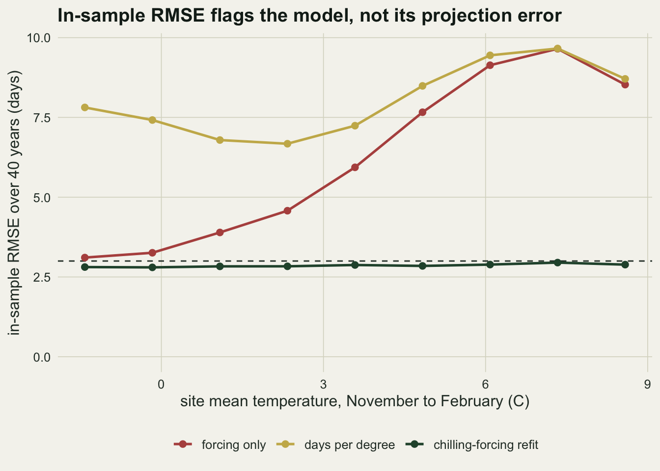
mc4 <- mc[mc$warm == 4, ]
mc4$err_known <- mc4$known - mc4$truth
fo_worse   <- mean(mc4$r_fo > mc4$r_known)
ratio_rmse <- a4$r_fo / a4$r_known
fit_worst  <- which.max(ratio_rmse)
gap_cor    <- cor(abs(gap4), a4$r_fo - a4$r_known)
stopifnot(fit_worst != worst, which.max(a4$r_fo) == fit_worst,
          abs(gap4[fit_worst]) < abs(gap4[worst]), gap_cor < 0)
mild4     <- mc4$site >= 6
edge_start <- sum(mc4$fo_start == max(fo_grid$start) & mild4)
edge_base  <- sum(mc4$fo_base == min(fo_grid$base) & mild4)
within2    <- tapply(abs(mc4$err_known) <= 2, mc4$site, sum)
err_lo     <- tapply(mc4$err_known, mc4$site, min)
err_hi     <- tapply(mc4$err_known, mc4$site, max)
wide       <- which.max(err_hi - err_lo)
stopifnot(err_lo[wide] <= -7, err_hi[wide] >= 7)
The chilling-forcing refit sits just under the observation error at every site, with a mean RMSE from 2.80 to 2.95 days. The forcing-only model is worse in 100 per cent of the 144 paired fits, and its mean RMSE rises from 3.11 days at the coldest site to 9.65 at the worst, 1.11 to 3.27 times the refit’s. The days-per-degree regression is poor everywhere, 6.7 to 9.7 days. So an in-sample comparison of a forcing-only fit with a chilling-forcing fit is a usable warning: where the forcing-only RMSE sits well above the observation error, and above a chilling model, its projections should not be trusted. The warning is weakest at the coldest site, where the RMSE gap is 0.30 days while the projection at plus 4 C is off by 4.2. Nor does the size of the gap measure the damage: the worst forcing-only fit, at 7.3 C (an RMSE 3.27 times the refit’s), belongs to a site where its plus 4 C projection is off by only 1.3 days, while the largest projection error, 16.6 days, comes with a ratio of 2.06. Over the nine sites the correlation between the RMSE gap and the size of the projection error is -0.27. The RMSE says the forcing-only model is wrong, not by how much.
The forcing-only fit also shows the strain in its own parameters. At the four mildest sites its start date lands on 1 April, the last date the grid allows and days before the tree’s mean leaf-out, in 35 of 64 fits, and its base temperature on 0 C, the lowest allowed, in 33. A fitted start at the edge of the grid is the model turning itself into a calendar rule, which is how a forcing-only model imitates a tree whose date hardly moves with spring warmth.
The shaded band in the sweep figure is the less comfortable part. The right model, refitted on one forty-year record, projects the plus 4 C change to within 2 days of the truth in only 59 of 144 fits. At the site with a winter mean of 2.3 C single-record errors run from -9.6 to +16.7 days, while at the coldest and mildest sites 13 and 15 of 16 fits are within 2 days. The chunk below checks whether that spread is an artefact of the coarse parameter grid, by refitting eight further records at that site on a grid twice as fine in each of a, b and c.
set.seed(4321)
fine <- do.call(rbind, lapply(1:8, function(r) {
  t_fit <- weather_anom(n_fit) + rep(clim_of(site_tab$t_ann[wide]), each = n_fit)
  y     <- leaf_out(t_fit) + round(rnorm(n_fit, 0, obs_sd))
  t_now <- anom_proj + rep(clim_of(site_tab$t_ann[wide]), each = n_proj)
  f_c <- fit_cf(t_fit, y, rules$known)
  f_f <- fit_cf(t_fit, y, rules$known, cg = seq(0.00625, 0.07875, by = 0.0025),
                bg = seq(125, 1975, by = 50), ag = seq(1.25, 298.75, by = 2.5))
  proj <- function(f) mean(pred_cf(f, t_now + 4)) - mean(pred_cf(f, t_now))
  data.frame(coarse = proj(f_c), fine = proj(f_f), b = f_f$b, c = f_f$c,
             chill_fit_min = min(chill_at_leaf(t_fit)))
}))
fine_err <- range(fine$fine - m4$shift[wide])
bc_cor   <- cor(fine$b, fine$c)
chill_w4 <- chill_at_leaf(anom_proj + rep(clim_of(site_tab$t_ann[wide]), each = n_proj) + 4)
share_below <- sapply(fine$chill_fit_min, function(m) mean(chill_w4 < m))
stopifnot(bc_cor > 0, min(share_below) > 0)
On the finer grid the eight projections still miss the truth by -10.8 to +11.2 days, so the spread is not the grid, though single records moved by up to 13.4 days between the two grids, another sign of how weakly one record pins down b and c. The fitted b and c move together, with a correlation of 0.92 over the eight fits: records that return a larger no-chill requirement also return a faster decay, and the projections part company because plus 4 C takes the site outside the chill range the records cover. The least-chilled year in each record had 42 to 76 chill days by leaf-out, against a present-climate mean of 114; at plus 4 C the mean is 47, and 44 to 88 per cent of the warmed winters have less chill than the least-chilled year of the record they are projected from. A projection from the right model is an extrapolation of its exponential, and one site’s record constrains that exponential only over the winters it has seen.
When the chill rule is wrong
The refit so far was handed the true chill rule. In a real analysis the rule is a choice: which temperatures count as chilling, and from when. Two plausible wrong rules are fitted to the same records. The first counts a bounded window, days with a mean from 0 to 7 C, from 1 November, so that frozen days no longer count and mild days up to 7 C do. The second keeps the right threshold but starts counting on 1 December.
mc4$err_window <- mc4$window - mc4$truth
mc4$err_late   <- mc4$late - mc4$truth
win_worse  <- mean(mc4$r_window > mc4$r_known)
win_vs_fo  <- tapply(mc4$r_window > mc4$r_fo, mc4$site, mean)
late_worse <- tapply(mc4$r_late > mc4$r_known, mc4$site, mean)
win_chill <- t(sapply(1:3, function(st) {
  t_now <- anom_proj + rep(clim_of(site_tab$t_ann[st]), each = n_proj)
  c(win_now = mean(chill_days(t_now, rules$window)[, apr30]),
    win_w4  = mean(chill_days(t_now + 4, rules$window)[, apr30]),
    true_now = mean(chill_days(t_now)[, apr30]),
    true_w4  = mean(chill_days(t_now + 4)[, apr30]))
}))
stopifnot(win_chill[1, "win_w4"] > win_chill[1, "win_now"],
          diff(win_chill[3, 2:1]) < diff(win_chill[3, 4:3]))
pick <- apply(mc4[, c("r_known", "r_window", "r_late")], 1, which.min)
mc4$picked   <- c("known", "window", "late")[pick]
mc4$err_pick <- ifelse(mc4$picked == "known", mc4$known,
                       ifelse(mc4$picked == "window", mc4$window, mc4$late)) - mc4$truth
pick_known <- tapply(mc4$picked == "known", mc4$site, sum)
pick_err   <- tapply(mc4$err_pick, mc4$site, mean)
n_window_picked <- sum(mc4$picked == "window")
late_gap   <- a4$late - a4$truth
late_z     <- abs(late_gap) / mse$late[mse$warm == 4]
diff_kl    <- abs(a4$known - a4$late)
stopifnot(max(late_gap) < 0, all(late_worse[5:9] == 1),
          all(pick_known[min(which(pick_known == n_rep)):9] == n_rep),
          a4$window[delay_sites[1]] < 0, which.max(diff_kl) > 2)
mis_panels <- c("change in leaf-out at plus 4 C (days)", "in-sample RMSE (days)")
mis_vars <- c("known", "window", "late", "truth", "r_known", "r_window", "r_late")
mis_long <- data.frame(winter = a4$winter, value = unlist(a4[mis_vars]),
model = factor(rep(sub("^r_", "", mis_vars), each = nrow(a4)),
c("known", "window", "late", "truth"),
c("right rule", "window 0 to 7 C", "counted from 1 December", "truth")),
panel = factor(rep(mis_panels[c(1, 1, 1, 1, 2, 2, 2)], each = nrow(a4)), mis_panels))
ggplot(mis_long, aes(winter, value, colour = model)) +
geom_hline(data = data.frame(panel = factor(mis_panels[1], mis_panels), yv = 0),
aes(yintercept = yv), colour = te_body, linewidth = 0.4) +
geom_line(aes(linetype = model), linewidth = 0.9) +
geom_point(size = 1.9) +
facet_wrap(~ panel, scales = "free_y") +
scale_colour_manual(values = c(te_forest, te_rust, te_gold, te_ink), name = NULL) +
scale_linetype_manual(values = c("solid", "solid", "solid", "22"), name = NULL) +
labs(x = "site mean temperature, November to February (C)", y = NULL,
title = "The chill rule decides the projection") +
theme_datasheet() +
theme(legend.position = "bottom", legend.key.width = unit(1.6, "lines"))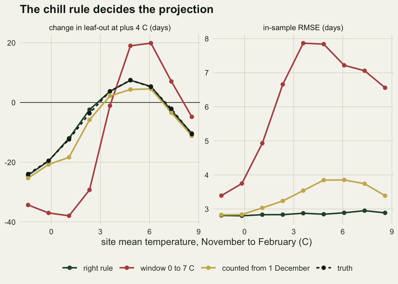
The window rule is badly wrong in projection. At the three coldest sites it projects advances of 34.3, 37.0 and 38.0 days against true advances of 24.0, 19.5 and 12.4, because under that rule warming turns frozen days into chill days. By 30 April the window count at the coldest site rises from 77 to 109 days while the true chill falls from 158 to 110, and at the third site it falls only from 103 to 93 while the true chill falls from 132 to 68. The fitted tree gains or keeps chill where the real one loses it. At two of the three delay sites the window rule overstates the delay, projecting +19.0 and +19.9 days where the truth is +7.5 and +5.2, and at the first it gets the sign wrong, -1.1 where the truth is +3.8. It does not hide, though. Its RMSE is higher than the right rule’s in 100 per cent of the 144 fits, and at the five coldest sites it is even higher than the forcing-only model’s in 81 to 100 per cent of fits. A chilling model that fits worse than a forcing-only one is evidence against its chill rule, not against chilling.
The late start is the harder case. Its projections are closer, with mean errors at plus 4 C from -6.0 to -0.6 days, all on the side of too much advance and largest at the site with a winter mean of 1.1 C. The Monte Carlo SE of these means is up to 1.7 days; the error is under one SE at 1 of the nine sites and over two at 5, and the sites share their weather, so the common sign is not nine independent checks. What makes it hard is the fit: at the two coldest sites its RMSE is higher than the right rule’s in only 44 and 56 per cent of fits; there the forty years cannot tell the two rules apart. From the site with a winter mean of 3.6 C upwards it is worse in every fit.
Choosing among the three rules by in-sample RMSE, as an analyst with no other information might, never picks the window rule (0 of 144 fits) and picks the right rule in 8 of 16 fits at the coldest site and in all 16 from the site with a winter mean of 3.6 C upwards. The mean error of the chosen model’s projection is within 1.4 days of the truth at every site. The window rule drops out on its fit. Between the other two the mean projections differ by 0.8 to 6.4 days across the sites, most at the site with a winter mean of 1.1 C, where the RMSE already favours the right rule in 14 of 16 fits; at the two coldest sites, where the forty years cannot tell them apart, the difference is 0.9 and 1.2 days.
What to report
Report the in-sample RMSE of a forcing-only model next to that of at least one chilling-forcing model, and next to the observation error of the dates. In this simulation the forcing-only RMSE exceeded the chilling model’s in every paired fit, and its site mean reached 3.3 times the chilling model’s; a forcing-only model whose error is far above the recording error of the dates is missing something, and chilling is one of the candidates. The comparison works in one direction only: a small gap, as at the coldest site here, does not guarantee a good projection, and a large one does not say how far off the projection is.
Report the fitted start date and base temperature of a forcing-only model, and say if either sits on the edge of the range searched. A start date days before the mean event is not a biological estimate.
Fit the chilling-forcing model under more than one chill rule, and treat a rule that fits worse than the others, or worse than forcing alone, as refuted by the record. Among rules that fit alike, report the spread of their projections rather than the one with the lowest RMSE: here the right rule and a rule starting a month late were often indistinguishable at the two coldest sites. The rule itself is better taken from experiments that chill and force cut twigs under control than from the leaf-out record.
Give the chill a site accumulates in the projected climate next to the range seen in the fitting years. When the projected winters lie outside that range, even the right model is extrapolating its chill response, and a single record’s projection can be off by a week or more in either direction, as the band in the sweep figure shows. A projection from one site needs an interval, and the obvious route, a bootstrap over years, was not tested here.
Quote a days-per-degree sensitivity as a description of the past, not as a projection. Where chilling matters it will not extrapolate, and its in-sample fit, poor everywhere, gives no guide to where it fails.
Honest limits
The tree follows one model form with one set of constants. The alternating form is one of several budburst models; in a sequential model forcing only starts once a chilling requirement is met, and the location and size of the delay region would differ. Those were not simulated, and the constants a, b and c were chosen to put leaf-out in spring and the chill threshold inside the sweep, not taken from a species. Warming here is a uniform shift of every day. Real warming is uneven, and a winter that warms faster than the spring removes more chill for the same added forcing than this sweep does; the reverse removes less. The sites differ only in mean temperature, with one seasonal amplitude, one weather generator and no between-tree variation beyond a 3 day observation error.
Daylength does not enter. Many trees need both chill and a long enough day, and a photoperiod limit would cap the advance at the cold end where this tree keeps advancing; see Daylength as a predictor in ecology for why daylength is hard to separate from day of year at one site.
The forcing-only model was searched over base temperatures from 0 to 8 C and start dates to 1 April, and at the mild sites it ran into both edges. A wider grid could give a different forcing-only model there; no grid gives it chill. The misspecified rules are two choices among many. A wrong threshold that is closer to the truth, a chill count weighted by temperature, or a start date that shifts from year to year would each give a different error, and the finding that in-sample RMSE removed the grossly wrong rule here is not a guarantee that it will remove every wrong rule.
All fits use one site’s record. Real calibrations often pool sites or years across a climate gradient, which widens the chill range the model sees and should narrow the single-record spread measured above; that was not measured. Nor does this post address whether chilling limits real trees as much as the model says: Gao and colleagues (2024) argue that field-calibrated models misstate it, and the simulation cannot speak to that.
References
Cannell MGR, Smith RI 1983 Journal of Applied Ecology 20(3):951-963 (10.2307/2403139)
Chuine I 2000 Journal of Theoretical Biology 207(3):337-347 (10.1006/jtbi.2000.2178)
Fu YH, Zhao H, Piao S, Peaucelle M, Peng S, Zhou G, Ciais P, Huang M, Menzel A, Penuelas J, Song Y, Vitasse Y, Zeng Z, Janssens IA 2015 Nature 526(7571):104-107 (10.1038/nature15402)
Gao X, Richardson AD, Friedl MA, Moon M, Gray JM 2024 Global Ecology and Biogeography 33(12):e13932 (10.1111/geb.13932)