library(ggplot2)

te_paper  <- "#f5f4ee"
te_ink    <- "#16241d"
te_body   <- "#2c3a31"
te_forest <- "#275139"
te_rust   <- "#b5534e"
te_gold   <- "#c9b458"
te_line   <- "#dad9ca"

theme_datasheet <- function() {
  theme_minimal(base_size = 12) +
    theme(plot.background  = element_rect(fill = te_paper, colour = NA),
          panel.background = element_rect(fill = te_paper, colour = NA),
          panel.grid.major = element_line(colour = te_line, linewidth = 0.3),
          panel.grid.minor = element_blank(),
          text             = element_text(colour = te_body),
          plot.title       = element_text(colour = te_ink, face = "bold"),
          plot.subtitle    = element_text(colour = te_body),
          axis.text        = element_text(colour = te_body))
}Chi-squared approximation may be incorrect
R
hypothesis testing
count data
statistics
ecology tutorial
What the chisq.test warning means for a small two by two table in R: exact sizes and power show Yates’ correction, not the warning, is what costs you power.
A dormouse survey hangs twenty nest boxes in a coppiced wood and twenty in the neighbouring high forest. At the end of the season six of the coppice boxes and one of the high forest boxes have held a nest. The two by two table goes into chisq.test(), and R returns a p value together with a line that is easy to scroll past: Chi-squared approximation may be incorrect. Some readers then switch to fisher.test(), some drop the warning into suppressWarnings(), and some report the p value anyway. The first choice changes the p value; the other two keep the corrected one. The warning itself says nothing about which to trust.
What the warning means has a precise answer, because a two by two table from two groups of fixed size has a finite sample space. Every possible table can be listed, each one has a probability under the null hypothesis that both groups share one occupancy rate, and the rate at which a test rejects is a finite sum over that list. Nothing before the last section is simulated: the sizes and powers are computed exactly, to rounding, so there are no seeds and no Monte Carlo errors attached to them. The result is not new. Campbell (2007) compared seven versions of the chi-square and Fisher-Irwin tests over a large grid of small two by two tables and recommended the ‘N-1’ chi-square of Pearson (1947) whenever the smallest expected count is at least one. This post agrees with it on the designs computed here, in base R at sample sizes that field ecologists actually have and with the limits set out below, and shows where the loss sits: in the continuity correction of Yates (1934), which chisq.test() applies to every two by two table unless told not to.
Four posts here run chi-square tests on counts, but in none of them does R print the warning. Hardy-Weinberg expectations in R sets a goodness of fit chi-square against an exact test on genotype counts, and on a rare allele the two disagree across the threshold, with the chi-square the one in error; its expected counts there are small enough to set the warning off, but the statistic is computed by hand and referred to pchisq(), and it is a one-sample test with no continuity correction in play. Log-linear models for three-way count tables calls chisq.test(tab2, correct = FALSE) on its collapsed two by two table without saying why the correction is switched off. Germination trials as time-to-event data computes the rejection rate of prop.test() by the same kind of finite sum over two binomial distributions used below, with the default correction left on; a chunk below checks that prop.test() on two groups is the same corrected test. And Checking your data against the design wraps a uniform goodness of fit chi-square on terminal digits in suppressWarnings(), which is a one-way table where the correction never applies (with 720 records each digit expects 72, so the warning cannot fire there). None of them asks what the correction costs, which is the subject here.
What chisq.test does to a two by two table
The nest box table first, run through the five tests this post compares. The uncorrected Pearson chi-square is chisq.test(x, correct = FALSE). The default call subtracts one half from every absolute deviation between observed and expected counts before squaring, which is Yates’ correction. The N-1 chi-square multiplies the uncorrected statistic by (N - 1) / N, where N is the total count; Pearson (1947) proposed it and Campbell (2007) tested it. Fisher’s test is fisher.test(), whose two-sided p value adds up the probabilities of every table with the same margins that is no more probable than the observed one (Irwin’s rule). The mid-p version of Lancaster (1961) counts only half of the probability of tables exactly as probable as the observed one; it is not in base R and is computed by hand below.
ex_a <- 6; ex_b <- 1; n_box <- 20
nest_tab <- matrix(c(ex_a, n_box - ex_a, ex_b, n_box - ex_b), 2,
                   dimnames = list(c("nest", "empty"), c("coppice", "high forest")))

ex_warned <- FALSE
p_default <- withCallingHandlers(chisq.test(nest_tab)$p.value,
  warning = function(w) { ex_warned <<- TRUE; invokeRestart("muffleWarning") })
ex_expected <- suppressWarnings(chisq.test(nest_tab)$expected)
ex_stat_unc <- unname(suppressWarnings(chisq.test(nest_tab, correct = FALSE)$statistic))
n_tot <- sum(nest_tab)
ex_p <- c(yates     = p_default,
          pearson   = suppressWarnings(chisq.test(nest_tab, correct = FALSE)$p.value),
          n_minus_1 = pchisq(ex_stat_unc * (n_tot - 1) / n_tot, 1, lower.tail = FALSE),
          fisher    = fisher.test(nest_tab)$p.value)
round(ex_p, 4)
yates pearson n_minus_1 fisher
0.0960 0.0375 0.0399 0.0915 The smallest expected count is 3.5, below five, so R warns. The default, corrected p value is 0.096 and Fisher’s is 0.091; the uncorrected chi-square gives 0.037 and the N-1 version 0.040. One table, two verdicts at the five per cent level. The rest of the post asks which pair of numbers is honest about its level.
Two statements about R need to hold for that question to make sense, and they are checked here rather than asserted. The warning is raised by one line in the source of chisq.test(), if (any(E < 5) && is.finite(PARAMETER)), which is the same line in R 4.3.3, where this post was run, and in the development source of R 4.7.0 read on the day of writing: it fires when any expected count is below five, whatever the table size. Five is the old rule of thumb that Campbell (2007) traces to Fisher and to Cochran (1954), applied here to every cell without exception. The correction is applied when correct = TRUE, the default, and the table is two by two; the subtracted amount is min(0.5, abs(x - E)), so it never overshoots a deviation smaller than one half. For a larger table nothing is subtracted.
stopifnot(isTRUE(formals(chisq.test)$correct), isTRUE(formals(prop.test)$correct))
stopifnot(ex_warned, any(ex_expected < 5))

# the corrected statistic is the uncorrected one with min(0.5, |O - E|) taken off
dev_ex  <- abs(nest_tab - ex_expected)
yat_man <- sum((dev_ex - min(0.5, dev_ex))^2 / ex_expected)
stopifnot(abs(unname(suppressWarnings(chisq.test(nest_tab)$statistic)) - yat_man) < 1e-10)

# prop.test on two groups is the same corrected test
stopifnot(abs(suppressWarnings(prop.test(c(ex_a, ex_b), c(n_box, n_box))$p.value) -
              ex_p["yates"]) < 1e-12)

# a two by three table gets no correction, with correct = TRUE left on
tab_23 <- matrix(c(9, 7, 4, 12, 5, 3), 3)
stopifnot(abs(suppressWarnings(chisq.test(tab_23)$statistic) -
              suppressWarnings(chisq.test(tab_23, correct = FALSE)$statistic)) < 1e-12)
Every table, every test, one function
Two groups of sizes n1 and n2, with a successes in the first and b in the second, give (n1 + 1)(n2 + 1) possible tables. The function below returns the five p values and the warning flag for all of them at once. The chi-square statistics have closed forms in a, b and the margins. Fisher’s test and the mid-p need the hypergeometric distribution of a given the total a + b, which is where the conditioning on the margins enters. A table with no successes or no failures at all has a zero margin, no test can say anything about it, and it is counted as not rejected; chisq.test() returns a missing p value for it, with the warning.
alpha_lev <- 0.05
tie_tol   <- 1e-7                    # the relative tolerance fisher.test uses for ties

tab_tests <- function(n1, n2) {
  tabs <- expand.grid(a = 0:n1, b = 0:n2)
  n_all <- n1 + n2
  k_suc <- tabs$a + tabs$b
  cross <- tabs$a * n2 - tabs$b * n1
  denom <- n1 * n2 * k_suc * (n_all - k_suc)
  x2 <- ifelse(denom > 0, n_all * cross^2 / denom, NA)
  dev_abs <- abs(cross) / n_all                    # |O - E|, the same in all four cells
  x2_yat <- ifelse(denom > 0, (dev_abs - pmin(0.5, dev_abs))^2 * n_all^3 / denom, NA)
  p_fis <- p_mid <- p_mid_dbl <- numeric(nrow(tabs))
  for (k in 0:n_all) {
    rows <- which(k_suc == k)
    a_rng <- max(0, k - n2):min(n1, k)
    dens <- dhyper(a_rng, n1, n2, k)
    for (i in rows) {
      d_obs <- dens[a_rng == tabs$a[i]]
      below <- dens < d_obs * (1 - tie_tol)
      tied  <- !below & dens <= d_obs * (1 + tie_tol)
      p_fis[i] <- sum(dens[below | tied])
      p_mid[i] <- sum(dens[below]) + 0.5 * sum(dens[tied])
      p_mid_dbl[i] <- min(1, 2 * min(sum(dens[a_rng < tabs$a[i]]) + d_obs / 2,
                                     sum(dens[a_rng > tabs$a[i]]) + d_obs / 2))
    }
  }
  min_exp <- min(n1, n2) * pmin(k_suc, n_all - k_suc) / n_all
  out <- data.frame(tabs, warn = min_exp < 5, min_exp = min_exp,
                    yates = pchisq(x2_yat, 1, lower.tail = FALSE),
                    pearson = pchisq(x2, 1, lower.tail = FALSE),
                    n_minus_1 = pchisq(x2 * (n_all - 1) / n_all, 1, lower.tail = FALSE),
                    fisher = p_fis, midp = p_mid, midp_dbl = p_mid_dbl)
  p_cols <- c("yates", "pearson", "n_minus_1", "fisher", "midp", "midp_dbl")
  out[p_cols][is.na(out[p_cols])] <- 1
  out$campbell <- ifelse(out$min_exp >= 1, out$n_minus_1, out$fisher)
  out
}

# check against R on all 441 tables of the 20 + 20 design
tt_20 <- tab_tests(20, 20)
r_side <- t(mapply(function(a, b) {
  m_ab <- matrix(c(a, 20 - a, b, 20 - b), 2)
  warned <- FALSE
  p_y <- withCallingHandlers(chisq.test(m_ab)$p.value,
    warning = function(w) { warned <<- TRUE; invokeRestart("muffleWarning") })
  c(warned, p_y, suppressWarnings(chisq.test(m_ab, correct = FALSE)$p.value),
    fisher.test(m_ab)$p.value)
}, tt_20$a, tt_20$b))
r_side[is.na(r_side)] <- 1
check_gap <- max(abs(r_side[, 2:4] - as.matrix(tt_20[c("yates", "pearson", "fisher")])))
stopifnot(all(r_side[, 1] == tt_20$warn), check_gap < 1e-10)
n_tab_20 <- nrow(tt_20)
On all 441 tables of a twenty plus twenty design the hand-written corrected, uncorrected and Fisher p values agree with chisq.test() and fisher.test() to within floating-point rounding (the stopifnot() above checks it), and the warning flag, computed as “any expected count below five”, matches the warning R actually raises on every table. The enumeration can therefore stand in for R’s own functions.
The size of each test, computed exactly
Under the null hypothesis both groups have the same success probability p. The probability of a particular table is the product of two binomial probabilities, and the size of a test is the sum of those products over the tables it rejects. This is the unconditional size: the two group sizes are fixed by the design, and the total number of successes is free to vary from one repeat of the study to the next, as it does in a nest box survey. The size depends on p, which the null hypothesis leaves unknown, so it is computed along a grid of p. All five tests give the same verdict when successes and failures are swapped, so the size at p equals the size at 1 - p and the grid stops at one half; a chunk below checks that symmetry on the unbalanced design.
designs <- data.frame(n1 = c(8, 12, 20, 30, 40, 60), n2 = c(8, 12, 20, 10, 40, 20))
p_grid  <- seq(0.02, 0.50, by = 0.01)
test_cols <- c("yates", "pearson", "n_minus_1", "fisher", "midp", "midp_dbl", "campbell")

rate_at <- function(tt, n1, n2, p1, p2 = p1) {
  w_tab <- dbinom(tt$a, n1, p1) * dbinom(tt$b, n2, p2)
  c(warn = sum(w_tab * tt$warn),
    vapply(tt[test_cols], function(p_val) sum(w_tab * (p_val < alpha_lev)), 0))
}

tt_list <- lapply(seq_len(nrow(designs)), function(i) tab_tests(designs$n1[i], designs$n2[i]))
size_tab <- do.call(rbind, lapply(seq_len(nrow(designs)), function(i) {
  n1 <- designs$n1[i]; n2 <- designs$n2[i]
  data.frame(design = sprintf("%d + %d", n1, n2), n1 = n1, n2 = n2, p = p_grid,
             t(vapply(p_grid, function(p0) rate_at(tt_list[[i]], n1, n2, p0), numeric(8))))
}))
size_tab$design <- factor(size_tab$design, levels = unique(size_tab$design))

# symmetry: size at p equals size at 1 - p, checked on the unbalanced 30 + 10 design
sym_gap <- max(abs(rate_at(tt_list[[4]], 30, 10, 0.2) - rate_at(tt_list[[4]], 30, 10, 0.8)))
stopifnot(sym_gap < 1e-12)

pick <- function(d, p0) size_tab[size_tab$design == d & abs(size_tab$p - p0) < 1e-9, ]
s20 <- pick("20 + 20", 0.15); s12 <- pick("12 + 12", 0.30)
s31 <- pick("30 + 10", 0.20); s08 <- pick("8 + 8", 0.50)
out_band <- size_tab$warn < 0.5
yates_max_out <- max(size_tab$yates[out_band])
pear_rng_out  <- range(size_tab$pearson[out_band])
pear_out_top  <- size_tab[out_band, ][which.max(size_tab$pearson[out_band]), ]
show_pts <- rbind(s08, s12, s20, s31)
show_tab <- data.frame(design = as.character(show_pts$design), p = show_pts$p,
warned = show_pts$warn, Yates = show_pts$yates,
Pearson = show_pts$pearson, "N-1" = show_pts$n_minus_1,
Fisher = show_pts$fisher, "mid-p" = show_pts$midp,
check.names = FALSE)
knitr::kable(show_tab, digits = c(0, 2, 3, 4, 4, 4, 4, 4), row.names = FALSE)| design | p | warned | Yates | Pearson | N-1 | Fisher | mid-p |
|---|---|---|---|---|---|---|---|
| 8 + 8 | 0.50 | 1.000 | 0.0213 | 0.0768 | 0.0529 | 0.0213 | 0.0255 |
| 12 + 12 | 0.30 | 0.848 | 0.0172 | 0.0492 | 0.0492 | 0.0172 | 0.0448 |
| 20 + 20 | 0.15 | 0.933 | 0.0120 | 0.0492 | 0.0492 | 0.0199 | 0.0350 |
| 30 + 10 | 0.20 | 1.000 | 0.0160 | 0.0437 | 0.0364 | 0.0235 | 0.0393 |
The table gives four points of the map. The column headed warned is the probability that the table a study ends up with makes R print the warning; the other columns are the probabilities of rejecting at the five per cent level when the null is true. At twenty boxes in each wood and an occupancy of 0.15, R warns on 93.3 per cent of the tables the survey could produce. On that design the uncorrected Pearson test rejects a true null in 0.0492 of studies, just under its nominal level, while the default corrected test rejects in 0.0120. At twelve plus twelve and p = 0.30 the pair is 0.0492 against 0.0172, and on the unbalanced thirty plus ten design at p = 0.20, where R warns on 100.0 per cent of tables, it is 0.0437 against 0.0160. Fisher’s test sits at or a little above the corrected test, at 0.0199, 0.0172 and 0.0235.
The first row of the table is the case that stops the advice from being “ignore the warning”. With eight units in each group and p = 0.50, the uncorrected test rejects a true null in 0.0768 of studies, which is liberal. The N-1 version brings that to 0.0529 and the mid-p to 0.0255.
size_long <- do.call(rbind, lapply(c("yates", "pearson", "n_minus_1", "fisher", "midp"), function(v)
  data.frame(design = size_tab$design, p = size_tab$p, size = size_tab[[v]], test = v)))
test_lab <- c(yates = "Yates (chisq.test default)", pearson = "Pearson, uncorrected",
              n_minus_1 = "N-1 chi-square", fisher = "Fisher", midp = "Fisher mid-p")
size_long$test <- factor(test_lab[size_long$test], levels = test_lab)
warn_band <- do.call(rbind, lapply(levels(size_tab$design), function(d) {
  sub_d <- size_tab[size_tab$design == d & size_tab$warn >= 0.5, ]
  if (nrow(sub_d) == 0) return(NULL)
  data.frame(design = d, lo = min(sub_d$p) - 0.005, hi = max(sub_d$p) + 0.005)
}))
warn_band$design <- factor(warn_band$design, levels = levels(size_tab$design))

ggplot(size_long, aes(p, size)) +
  geom_rect(data = warn_band, aes(xmin = lo, xmax = hi, ymin = -Inf, ymax = Inf),
            inherit.aes = FALSE, fill = te_line, alpha = 0.6) +
  geom_hline(yintercept = alpha_lev, linetype = "dashed", colour = te_body, linewidth = 0.5) +
  geom_line(aes(colour = test, linetype = test), linewidth = 0.8) +
  facet_wrap(~ design, ncol = 3) +
  scale_colour_manual(values = c(te_rust, te_ink, te_forest, te_gold, te_gold), name = NULL) +
  scale_linetype_manual(values = c("solid", "solid", "22", "solid", "42"), name = NULL) +
  labs(x = "common success probability p", y = "probability of rejecting a true null",
       title = "The correction bites inside the warning region and beyond it",
       subtitle = "grey: R warns on at least half the tables; dashed line: the nominal 0.05") +
  theme_datasheet() +
  theme(legend.position = "bottom") +
  guides(colour = guide_legend(nrow = 2))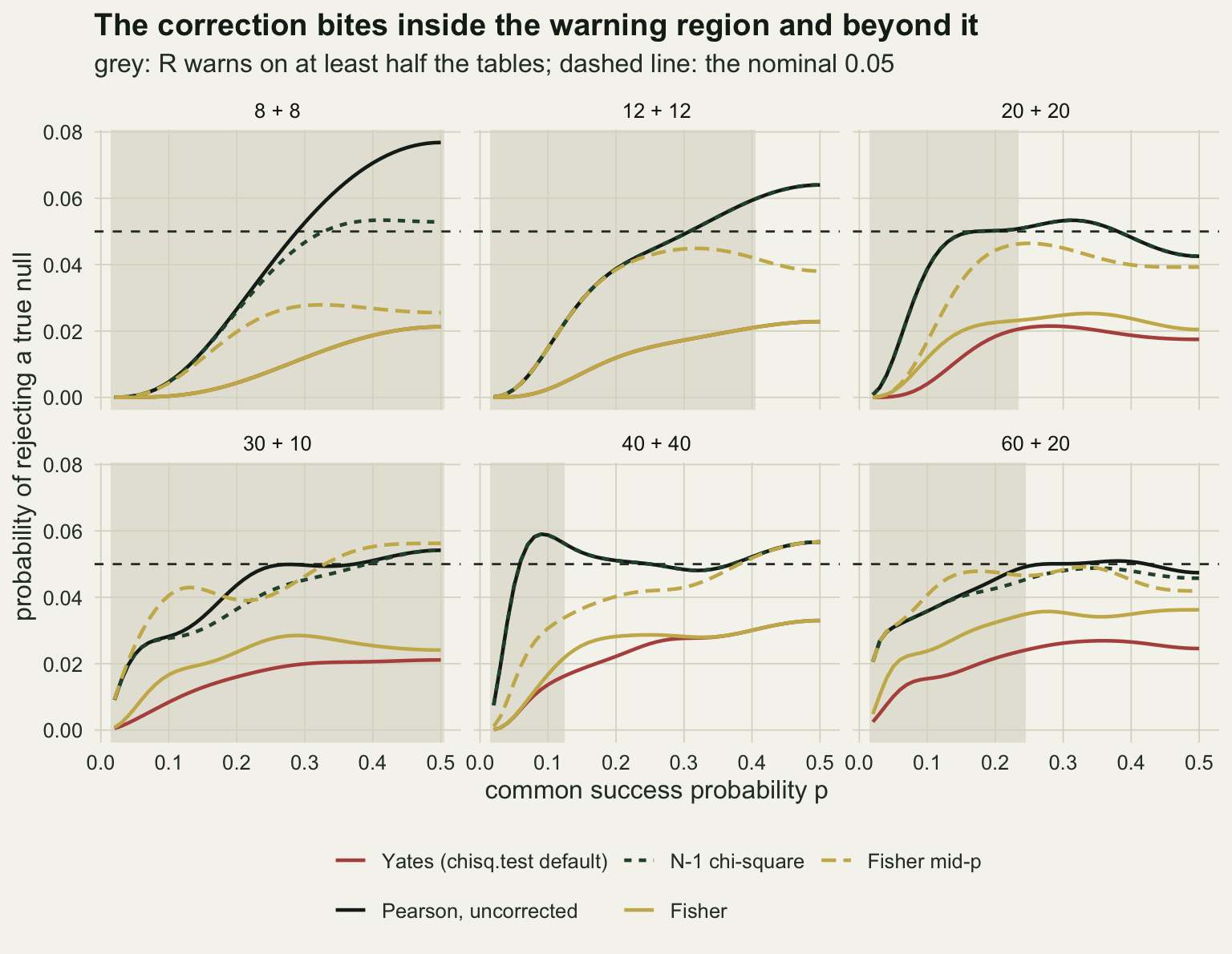
How much the correction costs where R warns
The figure puts the question the warning raises on one sheet. Inside the grey bands R warns on most of the tables a study could produce, and there the solid red line of the corrected test sits well under the dashed nominal level while the uncorrected and N-1 lines run near it, and above it in places. Outside the bands, at larger samples and less extreme p, the warning mostly stops and the uncorrected line stays between 0.0425 and 0.0640 (the top value at 12 + 12 and p = 0.50, where R still warns on 30.7 per cent of tables), but the corrected line does not come up to meet it: its largest size outside the bands is 0.0330. The correction is conservative well beyond the region the warning covers, and the warning is silent about that. The chunk below reads the whole grid rather than four points.
in_region <- size_tab$warn >= 0.5
reg <- size_tab[in_region, ]
n_reg <- nrow(reg); n_grid_all <- nrow(size_tab)
gap_reg <- reg$pearson - reg$yates
yates_below_all <- all(gap_reg > 0)
stopifnot(yates_below_all)
live <- reg$pearson >= alpha_lev / 2                # points where rejection is possible at all
n_live <- sum(live)
gap_live_min <- min(gap_live <- gap_reg[live]); gap_live_med <- median(gap_live)
ratio_live_med <- median(reg$yates[live] / reg$pearson[live])
yates_max_reg <- max(reg$yates)

alt_cols <- c("yates", "pearson", "n_minus_1", "midp", "campbell")
worst <- data.frame(
  test = c("Yates (default)", "Pearson, uncorrected", "N-1 chi-square", "Fisher mid-p", "Campbell's rule"),
  reg_max  = vapply(alt_cols, function(v) max(reg[[v]]), 0),
  reg_over = vapply(alt_cols, function(v) sum(reg[[v]] > alpha_lev), 0),
  reg_far  = vapply(alt_cols, function(v) sum(reg[[v]] > 1.1 * alpha_lev), 0),
  all_max  = vapply(alt_cols, function(v) max(size_tab[[v]]), 0),
  row.names = NULL)
w_of <- function(v) worst[alt_cols == v, ]
reg_row <- function(v) reg[which.max(reg[[v]]), ]
pear_reg <- reg_row("pearson"); mid_reg <- reg_row("midp")
camp_diff <- size_tab$n_minus_1 - size_tab$campbell
camp_gap <- max(abs(camp_diff)); camp_row <- size_tab[which.max(abs(camp_diff)), ]
camp_bal <- max(abs(camp_diff[size_tab$n1 == size_tab$n2]))
sparse_rej <- vapply(tt_list, function(tt) c(n1 = sum(tt$min_exp < 1 & tt$n_minus_1 < alpha_lev),
                                             fis = sum(tt$min_exp < 1 & tt$fisher < alpha_lev)), numeric(2))
n1_reg <- reg_row("n_minus_1")
mid_conv_gap <- max(abs(size_tab$midp - size_tab$midp_dbl))
mid_conv_row <- size_tab[which.max(abs(size_tab$midp - size_tab$midp_dbl)), ]

# what the correction's shortfall buys: the overshoot of the uncorrected test it prevents
short_reg <- alpha_lev - reg$yates; over_reg <- pmax(0, reg$pearson - alpha_lev); is_over <- over_reg > 0
short_ratio_med <- median(short_reg[is_over] / over_reg[is_over])
near_even <- reg[is_over & short_reg < 2 * over_reg, ]
stopifnot(sum(is_over) == w_of("pearson")$reg_over, all(near_even$design == "8 + 8"),
          max(near_even$p) == max(p_grid), nrow(near_even) == round((max(p_grid) - min(near_even$p)) / 0.01) + 1)
s08_short <- alpha_lev - s08$yates; s08_over <- s08$pearson - alpha_lev; s08_over_n1 <- s08$n_minus_1 - alpha_lev
# where (N - 1) / N changes a verdict, table by table; the N-1 worst cases; the mid-p on balanced designs
flip_n <- vapply(tt_list, function(tt) sum((tt$n_minus_1 < alpha_lev) != (tt$pearson < alpha_lev)), 0)
is_bal <- designs$n1 == designs$n2 & designs$n1 > 8
n1_top <- size_tab[which.max(size_tab$n_minus_1), ]
stopifnot(all(flip_n[is_bal] == 0), all(flip_n[!is_bal] > 0), n1_top$warn < 0.5,
          n1_reg$n1 == n1_reg$n2, n1_top$n1 == n1_top$n2)
tt_top <- tt_list[[which(designs$n1 == n1_top$n1 & designs$n2 == n1_top$n2)]]
top_rej_warned <- sum(dbinom(tt_top$a, n1_top$n1, n1_top$p) * dbinom(tt_top$b, n1_top$n2, n1_top$p) *
                      (tt_top$n_minus_1 < alpha_lev) * tt_top$warn)
mid_bal_over <- size_tab[size_tab$n1 == size_tab$n2 & size_tab$midp > alpha_lev, ]
stopifnot(all(mid_bal_over$design == "40 + 40"), max(mid_bal_over$warn) < 0.01)
mid40_top <- mid_bal_over[which.max(mid_bal_over$midp), ]knitr::kable(setNames(worst, c("test", "worst size, warning region", "points above 0.05",
"points above 0.055", "worst size, whole grid")),
digits = c(0, 4, 0, 0, 4), row.names = FALSE)| test | worst size, warning region | points above 0.05 | points above 0.055 | worst size, whole grid |
|---|---|---|---|---|
| Yates (default) | 0.0239 | 0 | 0 | 0.0330 |
| Pearson, uncorrected | 0.0768 | 58 | 30 | 0.0768 |
| N-1 chi-square | 0.0594 | 52 | 11 | 0.0640 |
| Fisher mid-p | 0.0563 | 18 | 11 | 0.0567 |
| Campbell’s rule | 0.0594 | 52 | 11 | 0.0640 |
Of the 294 combinations of design and p in the grid, 193 fall in the region where R warns on at least half the tables. The corrected test’s size is below the uncorrected test’s at every one of them. At the smallest p in each design no test can reject much, because tables with more than a few successes are rare, and there both sizes are close to zero; restricting to the 149 points where the uncorrected size is at least half the nominal level, the corrected test is lower by at least 0.0193 and by 0.0306 at the median point, and the median ratio of the two sizes is 0.35. Nowhere in the warning region does the corrected test’s size exceed 0.0239.
The other side matters as much, and the second table reads it off. The uncorrected test is not safe everywhere the warning fires: in the region it exceeds the nominal level at 58 of the 193 points and by more than a tenth of it at 30, with a worst case of 0.0768 at 8 + 8 and p = 0.50. The N-1 statistic removes the worst of that on the smallest design and has a worst case of 0.0594 in the region (12 + 12, p = 0.40); it exceeds the nominal level at 52 region points but by more than a tenth only at 11. The mid-p exceeds the nominal level at 18 region points, at most 0.0563 (30 + 10, p = 0.50). Campbell’s rule, the N-1 test when the smallest expected count is at least one and Fisher’s test otherwise, coincides with the plain N-1 test on the balanced designs (largest difference in size 0.0000), because no table with an expected count below one is rejected there by either. On each unbalanced design the N-1 test rejects up to 4 such tables and Fisher’s test up to 2, and at small p that makes Campbell’s rule the more conservative of the two, by up to 0.0160 in size (30 + 10, p = 0.05, where it gives 0.0068 against 0.0228). None of the alternatives holds the level exactly, and the uncorrected test is the one that strays furthest. At the 58 region points where it overshoots, the corrected test’s shortfall below 0.05 is at the median 6.2 times the overshoot it prevents, and at the other 135 there is no overshoot to prevent. Only at 8 + 8 from p = 0.38 upward is the shortfall less than twice the overshoot, and at p = 0.50 the two are about equal (0.0287 below against 0.0268 above); against the N-1 test’s overshoot at that point, 0.0029, the shortfall is 10 times larger.
A note on the mid-p. The two-sided version here subtracts half of the probability of the tables exactly as probable as the observed one from Fisher’s p value, which is Lancaster’s mid-p applied to Irwin’s ordering, the ordering fisher.test() uses. A common alternative doubles the smaller one-sided mid-p. With equal group sizes the two agree, because the hypergeometric distribution is symmetric; with unequal groups they do not, and the largest difference in size over the grid is 0.0243, at 30 + 10 and p = 0.12, where the doubled version gives 0.0184 against 0.0427; Fisher’s test itself gives 0.0183 there. A report that uses a mid-p should say which.
Fisher’s test is exact only given the margins
Fisher’s test is usually called exact, and in one sense it is: if the total number of successes is held at its observed value, the probability that the test rejects is never above five per cent. That is a statement about the conditional size, given the margins. The unconditional size, over studies whose totals vary, is an average of those conditional sizes weighted by how often each total occurs, and because the count a in the first group, given the total, can take only a few values, the conditional size is usually well below five per cent and often exactly zero.
n_c <- 20; n_all_c <- 2 * n_c; p_c <- 0.15
cond_tab <- do.call(rbind, lapply(0:n_all_c, function(k) {
  sub_k <- tt_20[tt_20$a + tt_20$b == k, ]
  dens_k <- dhyper(sub_k$a, n_c, n_c, k)
  data.frame(k = k, fisher = sum(dens_k * (sub_k$fisher < alpha_lev)),
             midp = sum(dens_k * (sub_k$midp < alpha_lev)),
             weight = dbinom(k, n_all_c, p_c))
}))
stopifnot(max(cond_tab$fisher) <= alpha_lev)
fis_uncond <- sum(cond_tab$weight * cond_tab$fisher)
route_gap  <- abs(fis_uncond - s20$fisher)
stopifnot(route_gap < 1e-12)
k_common <- cond_tab$k[cond_tab$weight >= 0.01]
k_zero   <- sum(cond_tab$fisher[cond_tab$k %in% k_common] == 0)
fis_cond_max <- max(cond_tab$fisher); mid_cond_max <- max(cond_tab$midp)
n_mid_cond_over <- sum(cond_tab$midp > alpha_lev)
w_mid_over <- sum(cond_tab$weight[cond_tab$midp > alpha_lev])
On the twenty plus twenty design, Fisher’s conditional size stays at or below five per cent for every total, as the construction guarantees; its largest value is 0.0484. Of the 11 totals that occur with probability at least 0.01 when p = 0.15, 4 have a conditional size of exactly zero: with those margins no table is extreme enough to reject. Averaging over the totals gives 0.0199, the unconditional size in the table above, reached this time by a second route (the two agree to within floating-point rounding). The mid-p gives up the conditional guarantee: its conditional size is above five per cent at 10 of the 41 possible totals, reaching 0.0915, and at p = 0.15 those totals together carry probability 0.194. In exchange its unconditional size is 0.0350 against Fisher’s 0.0199.
cond_show <- cond_tab[cond_tab$k <= 20, ]
cond_long <- rbind(data.frame(k = cond_show$k, size = cond_show$fisher, test = "Fisher"),
                   data.frame(k = cond_show$k, size = cond_show$midp, test = "Fisher mid-p"))
w_scale <- 0.05 / max(cond_show$weight)
ggplot(cond_long, aes(k, size)) +
  geom_col(data = cond_show, aes(k, weight * w_scale), inherit.aes = FALSE,
           fill = te_line, width = 0.8) +
  geom_hline(yintercept = alpha_lev, linetype = "dashed", colour = te_body, linewidth = 0.5) +
  geom_line(aes(colour = test, linetype = test), linewidth = 0.8) +
  geom_point(aes(colour = test), size = 2) +
  scale_colour_manual(values = c(te_gold, te_ink), name = NULL) +
  scale_linetype_manual(values = c("solid", "22"), name = NULL) +
  scale_y_continuous(sec.axis = sec_axis(~ . / w_scale, name = "probability of the total (grey)")) +
  labs(x = "total number of occupied boxes, both woods", y = "conditional size",
       title = "Exact given the margins, conservative on average",
       subtitle = "dashed line: 0.05; grey columns: how often each total occurs at p = 0.15") +
  theme_datasheet() +
  theme(legend.position = "bottom",
        axis.title.y.right = element_text(margin = margin(l = 8)))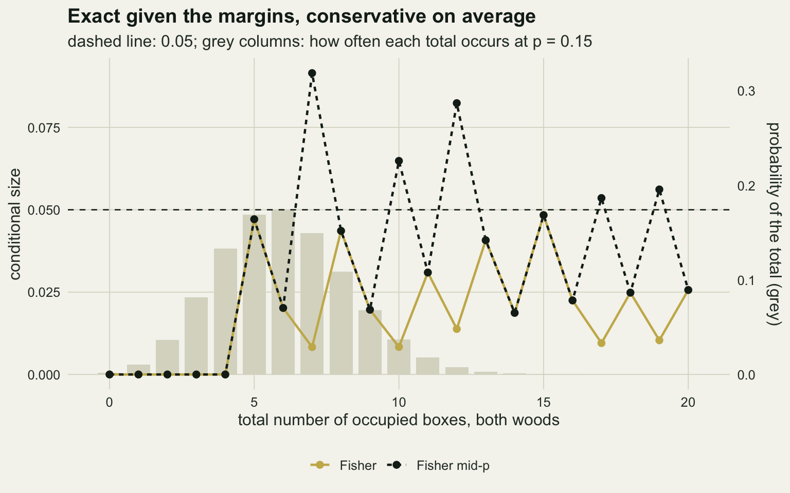
The price in power
A conservative test loses power, and the loss can be computed exactly in the same way, with the two groups given different success probabilities. The first comparison keeps twenty boxes per wood, an occupancy of 0.10 in the high forest, and lets the coppice rate rise.
p_base <- 0.10
p_alt_grid <- seq(0.10, 0.60, by = 0.02)
pow_tab <- data.frame(p2 = p_alt_grid,
  t(vapply(p_alt_grid, function(p2) rate_at(tt_20, 20, 20, p_base, p2), numeric(8))))
pw_a <- rate_at(tt_20, 20, 20, 0.10, 0.35)
tt_12 <- tt_list[[2]]
pw_b <- rate_at(tt_12, 12, 12, 0.15, 0.60)
pow_loss_a <- 1 - pw_a["yates"] / pw_a["pearson"]
pow_loss_b <- 1 - pw_b["yates"] / pw_b["pearson"]
With twenty boxes per wood and occupancies of 0.10 against 0.35, R warns on 59.0 per cent of the tables. The uncorrected test detects the difference in 0.491 of studies and the N-1 test in 0.491, the corrected default in 0.342, Fisher’s test in 0.361 and the mid-p in 0.476. The correction gives up 30 per cent of the power of the uncorrected test. At twelve per group with 0.15 against 0.60 the figures are 0.681 uncorrected, 0.507 corrected, 0.507 for Fisher and 0.634 for the mid-p, a loss of 25 per cent from the correction.
pow_long <- do.call(rbind, lapply(c("yates", "pearson", "n_minus_1", "fisher", "midp"), function(v)
  data.frame(p2 = pow_tab$p2, power = pow_tab[[v]], test = v)))
pow_long$test <- factor(test_lab[pow_long$test], levels = test_lab)
ggplot(pow_long, aes(p2, power)) +
  geom_vline(xintercept = 0.35, linetype = "dotted", colour = te_body, linewidth = 0.5) +
  geom_line(aes(colour = test, linetype = test), linewidth = 0.8) +
  scale_colour_manual(values = c(te_rust, te_ink, te_forest, te_gold, te_gold), name = NULL) +
  scale_linetype_manual(values = c("solid", "solid", "22", "solid", "42"), name = NULL) +
  labs(x = "coppice occupancy (high forest fixed at 0.10)", y = "probability of rejecting",
       title = "The corrected test needs a larger difference",
       subtitle = "twenty boxes per wood; dotted line: the 0.35 point quoted in the text") +
  theme_datasheet() +
  theme(legend.position = "bottom") +
  guides(colour = guide_legend(nrow = 2))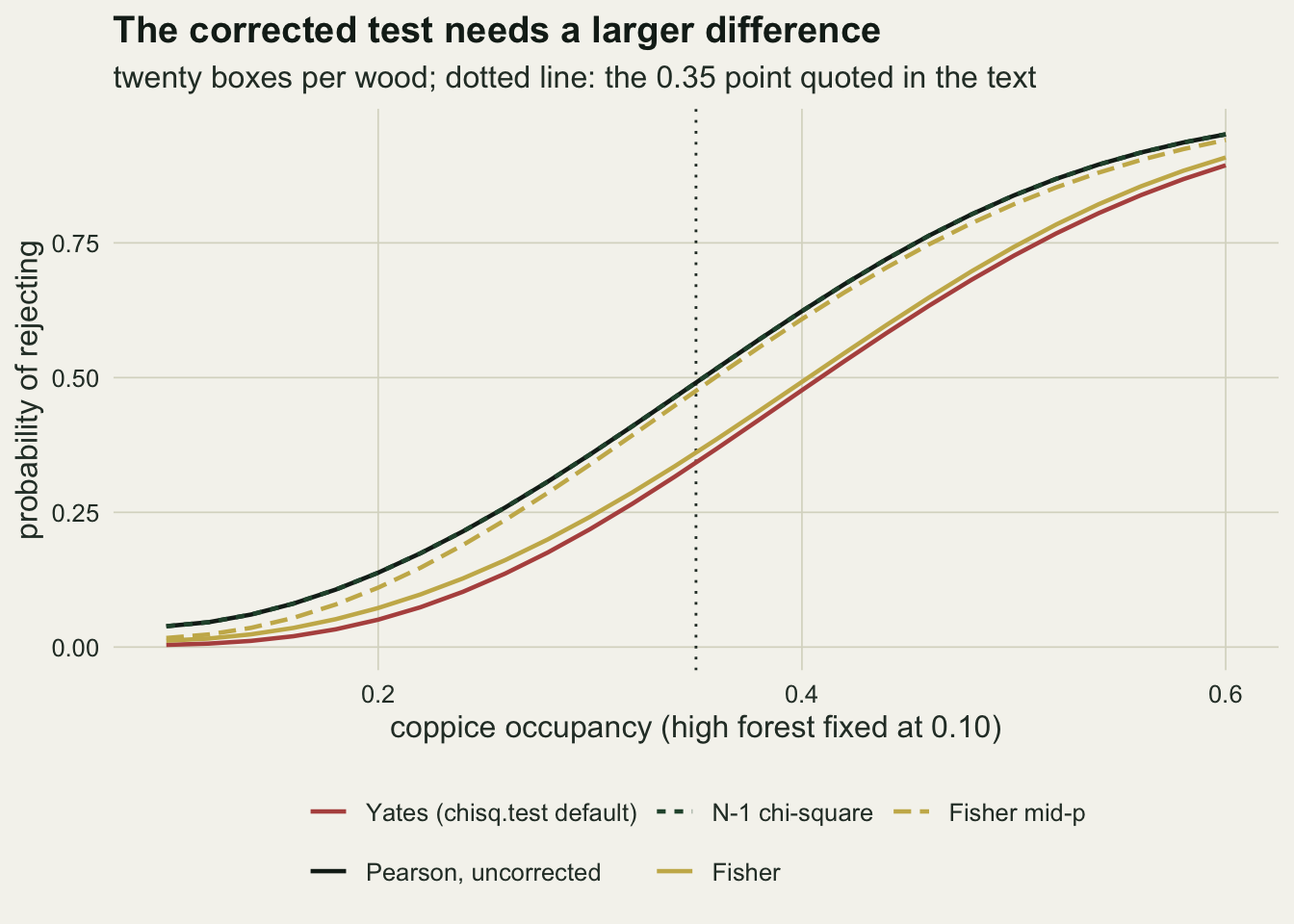
Larger tables get no correction
Everything above concerns the two by two case, because that is the only one in which chisq.test() changes the statistic. A two by three table with a rare category, say nest, roost and empty, gets the same warning and no correction. Its sample space of 53361 tables (each group of twenty falls into one of 231 splits over three categories) could be listed too; this part is simulated to show the Monte Carlo route, with the replication fixed before the run.
n_sim <- 40000; n_grp <- 20; p_cat <- c(0.7, 0.2, 0.1)
# the enumerable alternative: splits of one group over three categories, squared
stopifnot(sum(rowSums(expand.grid(0:n_grp, 0:n_grp, 0:n_grp)) == n_grp) == choose(n_grp + 2, 2))
set.seed(2031)
g_one <- rmultinom(n_sim, n_grp, p_cat); g_two <- rmultinom(n_sim, n_grp, p_cat)
row_tot <- g_one + g_two
empty_row <- colSums(row_tot == 0) > 0
level_grid <- c(0.01, 0.025, 0.05, 0.10)
rxc_p <- t(vapply(seq_len(n_sim), function(i) {
  m_i <- cbind(g_one[, i], g_two[, i])
  m_i <- m_i[rowSums(m_i) > 0, , drop = FALSE]      # chisq.test needs the empty row dropped
  warned <- FALSE
  p_chi <- withCallingHandlers(chisq.test(m_i)$p.value,
    warning = function(w) { warned <<- TRUE; invokeRestart("muffleWarning") })
  c(warned, p_chi, fisher.test(m_i)$p.value)
}, numeric(3)))
stopifnot(is.na(suppressWarnings(chisq.test(cbind(c(15, 5, 0), c(14, 6, 0)))$p.value)))
rxc_warn <- mean(rxc_p[, 1])
rxc_rate <- sapply(level_grid, function(l) c(pearson = mean(rxc_p[, 2] < l),
                                            fisher = mean(rxc_p[, 3] < l)))
rxc_se   <- sqrt(rxc_rate * (1 - rxc_rate) / n_sim)
i05 <- which(level_grid == alpha_lev)
share_empty <- mean(empty_row)
With twenty units per group and category probabilities of 0.7, 0.2, 0.1, R warns on 99.4 per cent of the 40000 simulated tables. The Pearson test rejects a true null in 0.0405 of them (Monte Carlo standard error 0.0010) and Fisher’s test in 0.0413 (standard error 0.0010). In 1.4 per cent of the draws the rare category was empty in both groups; chisq.test() returns a missing p value for a table with an empty row, so the row was dropped as a user would drop it, and the two by two remainder then does receive the correction. Both tests are somewhat conservative at this design, by a similar amount, and neither comes close to the loss that the correction causes on a two by two table with the same group sizes.
rxc_df <- data.frame(level = rep(level_grid, each = 2), test = rep(c("Pearson (chisq.test)", "Fisher"), 4),
                     rate = as.vector(rxc_rate), se = as.vector(rxc_se))
ggplot(rxc_df, aes(level, rate, colour = test)) +
  geom_abline(slope = 1, intercept = 0, linetype = "dashed", colour = te_body, linewidth = 0.5) +
  geom_errorbar(aes(ymin = rate - 2 * se, ymax = rate + 2 * se), width = 0.002,
                position = position_dodge(width = 0.004), linewidth = 0.5) +
  geom_point(size = 2.4, position = position_dodge(width = 0.004)) +
  scale_colour_manual(values = c(te_gold, te_ink), name = NULL) +
  scale_x_continuous(breaks = level_grid) +
  labs(x = "nominal level", y = "rejection rate under the null",
       title = "A larger table: no correction, mild conservatism",
       subtitle = "dashed line: rejection rate equal to the nominal level") +
  theme_datasheet() +
  theme(legend.position = "bottom")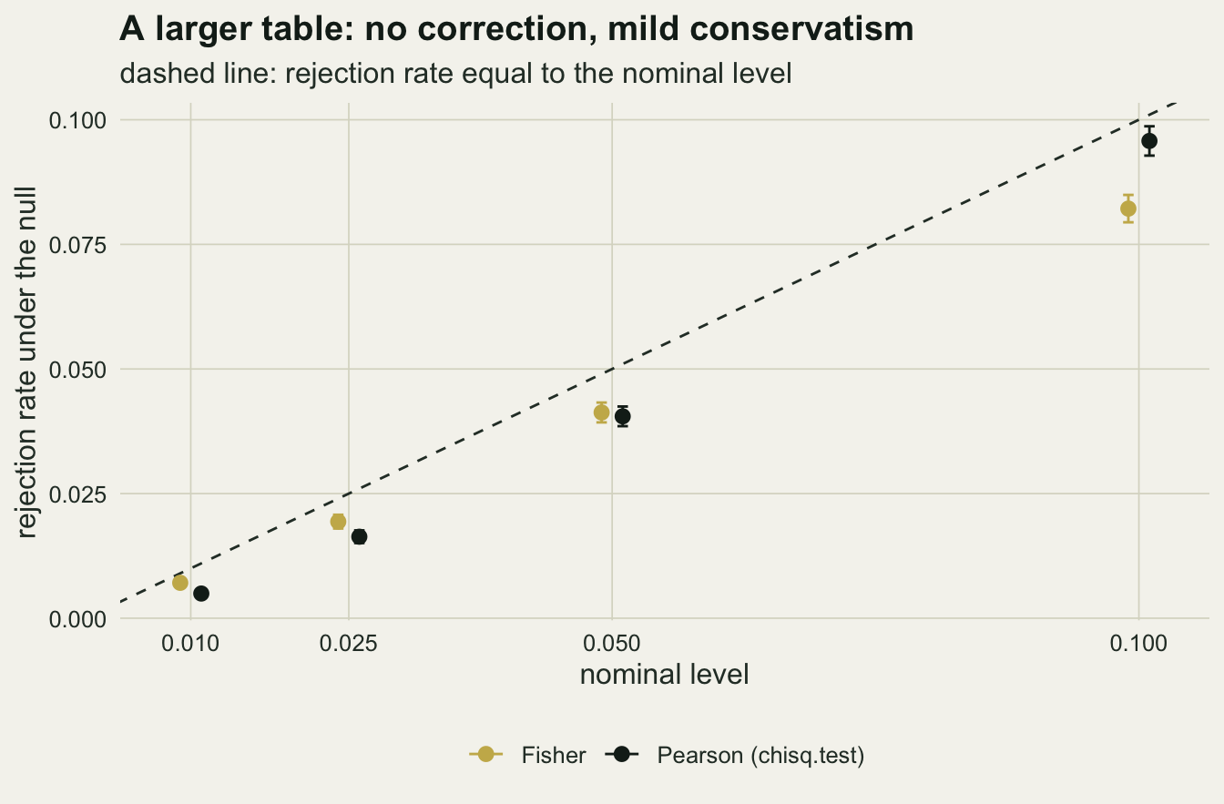
What to report
For a two by two table from two groups of fixed size, report the test by name. “A chi-square test” is ambiguous in R, because the default call is Yates-corrected and the output line that says so is easy to lose when the p value is copied out. If the analysis used the default, say “chi-square with Yates’ continuity correction”; if it used correct = FALSE, say “uncorrected Pearson chi-square”.
When R warns on a two by two table, the warning is not a reason to switch to a more conservative test, and it is not a reason to drop the correction silently either. Where R warned on most tables in the grid computed here, the N-1 chi-square reached at most 0.0594 and the mid-p at most 0.0563, while the default corrected test reached at most 0.0239, under half the nominal level. The uncorrected test is the one to avoid at the smallest samples, where it reached 0.0768. The N-1 statistic is one line of R: chisq.test(x, correct = FALSE)$statistic * (N - 1) / N referred to a chi-square with one degree of freedom. Campbell’s rule adds Fisher’s test for tables where some expected count is below one. Give the smallest expected count with the result, so that a reader can see which regime the table was in.
Neither the N-1 test nor the mid-p holds the level on every design. On the balanced designs of twelve, twenty and forty per group the N-1 test rejects exactly the tables the uncorrected test rejects, so its size there is the uncorrected size: up to 0.0594 inside the warning region (12 + 12, p = 0.40) and 0.0640 outside it (12 + 12, p = 0.50, where R still warns on 30.7 per cent of tables). The factor (N - 1) / N changes the verdict on some tables only at eight per group and on the two unbalanced designs. The mid-p stays below the nominal level on every balanced design except forty per group from p = 0.39 upward, far outside the warning region, where it reaches 0.0567, level with the uncorrected test. All these sizes average over every table a study could produce at a given p, warned or not: of the 0.0640 at 12 + 12 and p = 0.50, the tables on which R warns contribute 0.0197. The mid-p meant here is Fisher’s p value minus half the probability of the tables exactly as probable as the observed one; the version that doubles the smaller one-sided mid-p can be almost exactly as conservative as Fisher’s test on an unbalanced design (30 + 10, p = 0.12: 0.0184 against 0.0183).
If Fisher’s test is used, call it a conditional test, not an exact-size test. Its level is guaranteed given the margins; over repeats of a study with two groups of fixed size its size is below the nominal level, here 0.0199 at twenty plus twenty and p = 0.15. For the two by three table computed here, chisq.test() applied no correction and the warning marked a much smaller problem; fisher.test() or chisq.test(x, simulate.p.value = TRUE) are the usual alternatives, and a size computation of the kind above, by enumeration or by simulation, settles which is closer to the level at the sample size in hand.
Honest limits
The sizes are exact, but only for the sampling scheme computed: two independent groups of fixed size, which is the product binomial. A survey that fixes only the total number of units and cross-classifies them, or one that fixes both margins by design, has a different sample space and different sizes. Fisher’s conditional guarantee is the natural one when both margins are fixed; with only the group sizes fixed, as here, it holds given the observed total but not over repeats of the study.
The grid covers six designs and success probabilities from 0.02 to 0.5. The worst cases quoted for the uncorrected, N-1 and mid-p tests are maxima over that grid, not over every design; Campbell’s wider comparison is the source for the general recommendation, and a design outside the range here, such as three plus thirty, can behave differently. The alternatives computed are two points and one curve; a power statement for another design needs its own sum, which the function above provides.
All tests are two-sided at the five per cent level. At a one-sided or a stricter level the discreteness of the sample space weighs more, and the ordering of the tests is not guaranteed to be the same. The unconditional exact tests of Barnard and Boschloo, which maximise over the nuisance probability and so never exceed their level for any value of it, are not in base R and are not compared here; Lydersen, Fagerland and Laake (2009) review them alongside the tests above and report that Fisher’s test with the mid-p adjustment gives results close to those of an unconditional test.
The two by three part is a single simulated design with one rare category. It shows that chisq.test() applies no correction to a larger table and that its size held at that design; it does not map the size of the Pearson test over sparse larger tables, which can be liberal when many cells expect far less than one.
References
Campbell I 2007 Statistics in Medicine 26(19):3661-3675 (10.1002/sim.2832)
Yates F 1934 Journal of the Royal Statistical Society Series B 1(2):217-235 (10.2307/2983604)
Pearson ES 1947 Biometrika 34(1-2):139-167 (10.1093/biomet/34.1-2.139)
Lancaster HO 1961 Journal of the American Statistical Association 56(294):223-234 (10.1080/01621459.1961.10482105)
Cochran WG 1954 Biometrics 10(4):417-451 (10.2307/3001616)
Lydersen S, Fagerland MW, Laake P 2009 Statistics in Medicine 28(7):1159-1175 (10.1002/sim.3531)