library(ggplot2)
library(patchwork)

te_paper  <- "#f5f4ee"
te_ink    <- "#16241d"
te_body   <- "#2c3a31"
te_forest <- "#275139"
te_rust   <- "#b5534e"
te_gold   <- "#c9b458"
te_line   <- "#dad9ca"

theme_datasheet <- function() {
  theme_minimal(base_size = 12) +
    theme(plot.background  = element_rect(fill = te_paper, colour = NA),
          panel.background = element_rect(fill = te_paper, colour = NA),
          panel.grid.major = element_line(colour = te_line, linewidth = 0.3),
          panel.grid.minor = element_blank(),
          text             = element_text(colour = te_body),
          plot.title       = element_text(colour = te_ink, face = "bold"),
          plot.subtitle    = element_text(colour = te_body),
          axis.text        = element_text(colour = te_body),
          strip.text       = element_text(colour = te_ink))
}Biotic index scores and sorting effort
R
bioassessment
monitoring
freshwater
simulation
ecology tutorial
Average-score biotic indices drift with the number of animals sorted when sensitive families are rarer, so clean sites get flagged. Measured in R, with repairs.
A regional monitoring programme kick-samples forty riffles each spring and, as North American programmes and some European ones do, subsamples each sample in the laboratory to a fixed count of animals before identifying them to family. The reference sites were processed in a good year: the laboratory picked five hundred animals from every tray before stopping. This year the budget covers one hundred animals per sample. Each family on the programme’s list carries a tolerance score from 1 (survives almost anything) to 10 (needs clean, well oxygenated water), in the manner of the British BMWP scores; a BMWP-style index adds the scores of the families recorded, and an ASPT-style index divides that sum by the number of families. The average is the number that goes into the impairment decision, because it is usually described as the one that does not care how hard the sample was worked: a sum grows with every extra family found, an average of scores should not.
That description holds only if the families found late are a fair draw of the families found early. Picking stops at a count, so the families that turn up first are the abundant ones, and a family is missed at one hundred animals mainly because it is rare. If the sensitive families are also, on the whole, the rarer ones at a site, the first hundred animals over-represent tolerant families and the average score climbs as sorting continues. That condition carries the whole drift result, and no published estimate of the slope linking a family’s abundance to its tolerance score was found for this post. The drift is therefore measured at four assumed slopes, one of them zero; only the zero-slope results stand without the assumption. The post then measures what it does to a threshold set from references sorted to a larger count, and compares two ways to put the test site and the references back on the same footing.
None of the ingredients is new. Armitage and colleagues examined the BMWP score and its average per taxon, ASPT, over a wide range of unpolluted running-water sites, and found that replicate samples added substantially to the score but had little effect on ASPT. That is the only test of sampling effort on ASPT itself among the sources cited here, and at the sizes of whole-sorted UK samples it points against a large drift (see Honest limits). Lorenz and colleagues subsampled German stream samples electronically and found that, for the indices of the German AQEM assessment system, more than 40 per cent of 100-individual subsamples fell in a different quality class from the full sample, against under 20 per cent of 700-individual subsamples; that is a statement about variability between subsamples, not about a drift in one direction. Vinson and Hawkins showed that sampling area and the choice of fixed-count subsampling change taxon richness comparisons between streams; Barbour and Gerritsen defended fixed counts precisely because they standardise effort across samples. What follows is a demonstration, with a simulated family pool, of how those pieces combine for a score average and a percentile threshold.
This site has two neighbours that each hold one of the pieces still. Reference sites and tolerance bounds builds impairment thresholds from reference scores and, under “The false alarm rate belongs to the reference set”, scores those thresholds against test sites measured the same way as the references; sorting effort never varies there. Rarefaction and accumulation curves in R and Coverage-based rarefaction and extrapolation standardise effort, but for species richness, a count. Here the index is an average, the threshold comes from a reference set, and the only thing that differs between test site and references is how many animals were picked.
A family pool in which sensitive families are rarer
The pool has 70 families, seven at each score from 1 to 10. At an unimpaired site each family is present independently with probability 0.6, so sites differ in which families they hold as well as in how many animals of each. A present family gets a lognormal abundance whose log mean moves by b for every score unit above the pool middle of 5.5, with a log-scale standard deviation of 1.5 around it. The slope b is the assumption the post turns on. At b = 0 score and abundance are unrelated. At b = -0.25 a typical score-10 family has exp(-2.25), a little over a tenth, of the abundance of a typical score-1 family, with a great deal of scatter. The slopes 0, -0.1, -0.25 and -0.4 were fixed before any run, as were all other constants in the chunk.
Sorting is picking animals at random from the site until a count is reached. Picks are drawn as a sequence, so the first 100 animals of a sample are also the first 100 of its first 500: one simulated tray serves every count from 50 to 1000, and rarefying a larger sample down to a smaller count is exactly taking a shorter prefix of it. An impaired site halves the presence probability of the families scoring 7 to 10 and leaves everything else as it was.
n_fam     <- 70
score     <- rep(1:10, each = 7)            # tolerance score of each family
psi_clean <- 0.6                            # presence probability, unimpaired
psi_hit   <- 0.3                            # presence of scores 7 to 10, impaired
hit_from  <- 7
sd_log    <- 1.5                            # log-abundance scatter among families
slopes    <- c(0, -0.1, -0.25, -0.4)        # log-abundance change per score unit
n_grid    <- c(50, 100, 200, 300, 500, 1000)
n_ref     <- 500                            # animals sorted at reference sites
n_common  <- 100                            # common count for the blanket repair
q_flag    <- 0.10                           # reference percentile used as threshold
sens_cut  <- 8                              # sensitive family: score 8 or more
n_refsite <- 10000                          # reference sites per slope
n_sites   <- 4000                           # unimpaired and impaired test sites

sort_sites <- function(n_s, b, psi_vec) {
  n_max <- max(n_grid)
  aspt <- bmwp <- pct_sens <- matrix(NA_real_, n_s, length(n_grid))
  true_aspt <- true_bmwp <- true_sens <- numeric(n_s)
  for (i in seq_len(n_s)) {
    present  <- runif(n_fam) < psi_vec
    abund    <- present * exp(b * (score - 5.5) + rnorm(n_fam, 0, sd_log))
    picked   <- sample.int(n_fam, n_max, replace = TRUE, prob = abund)
    first_at <- match(seq_len(n_fam), picked, nomatch = n_max + 1)
    sens_run <- cumsum(score[picked] >= sens_cut)
    for (j in seq_along(n_grid)) {
      seen <- first_at <= n_grid[j]
      aspt[i, j] <- mean(score[seen])
      bmwp[i, j] <- sum(score[seen])
    }
    pct_sens[i, ] <- sens_run[n_grid] / n_grid
    true_aspt[i]  <- mean(score[present])
    true_bmwp[i]  <- sum(score[present])
    true_sens[i]  <- sum(abund[score >= sens_cut]) / sum(abund)
  }
  list(aspt = aspt, bmwp = bmwp, pct_sens = pct_sens,
       true_aspt = true_aspt, true_bmwp = true_bmwp, true_sens = true_sens)
}

psi_ref <- rep(psi_clean, n_fam)
psi_imp <- ifelse(score >= hit_from, psi_hit, psi_clean)
col_of <- function(n) match(n, n_grid)set.seed(20260910)
runs <- lapply(slopes, function(b) list(
ref = sort_sites(n_refsite, b, psi_ref),
test = sort_sites(n_sites, b, psi_ref),
hit = sort_sites(n_sites, b, psi_imp)))
names(runs) <- as.character(slopes)Each slope gets 10000 reference sites and 4000 unimpaired and 4000 impaired test sites, all unimpaired sites drawn from the same population. The function returns three indices at every count: the BMWP-like sum, the ASPT-like average, and, for contrast, the share of animals (not families) that belong to families scoring 8 or more. It also returns the value each index would take if every animal at the site were sorted: the sum and average over all present families, and the true abundance share of sensitive families.
The sum climbs, and so does the average
index_names <- c("BMWP-like sum", "ASPT-like average", "sensitive share of animals")
drift_tab <- do.call(rbind, lapply(seq_along(slopes), function(k) {
  tst <- runs[[k]]$test
  data.frame(slope = slopes[k], n = rep(n_grid, 3),
             index = rep(index_names, each = length(n_grid)),
             mean_value = c(colMeans(tst$bmwp), colMeans(tst$aspt),
                            colMeans(tst$pct_sens)),
             ratio = c(colMeans(tst$bmwp) / mean(tst$true_bmwp),
                       colMeans(tst$aspt) / mean(tst$true_aspt),
                       colMeans(tst$pct_sens) / mean(tst$true_sens)))
}))
dr <- function(b, n, idx, what = "mean_value") {
  drift_tab[[what]][drift_tab$slope == b & drift_tab$n == n & drift_tab$index == idx]
}
true_aspt_mean <- sapply(runs, function(r) mean(r$test$true_aspt))
sens_ratio_rng <- range(drift_tab$ratio[drift_tab$index == index_names[3]])
aspt_flat_rng  <- range(drift_tab$ratio[drift_tab$index == index_names[2] &
                                        drift_tab$slope == 0])
slope_cols <- c("0" = te_ink, "-0.1" = te_forest, "-0.25" = te_gold, "-0.4" = te_rust)
drift_tab$slope_f <- factor(as.character(drift_tab$slope), levels = names(slope_cols))
drift_tab$index_f <- factor(drift_tab$index, levels = index_names)
ggplot(drift_tab, aes(n, ratio, colour = slope_f)) +
geom_hline(yintercept = 1, linetype = "dashed", colour = te_body) +
geom_line(linewidth = 0.8) +
geom_point(size = 1.8) +
facet_wrap(~ index_f, nrow = 1) +
scale_x_log10(breaks = n_grid) +
scale_colour_manual(values = slope_cols, name = "slope b") +
labs(x = "animals sorted", y = "mean index / whole-site value") +
theme_datasheet() +
theme(legend.position = "bottom",
axis.text.x = element_text(angle = 45, hjust = 1))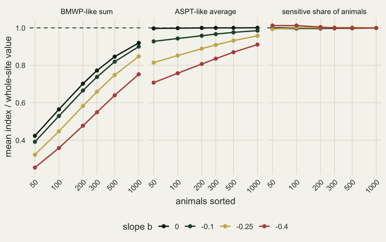
The sum behaves as expected of anything that counts families. With no abundance-tolerance link it reaches 0.565 of its whole-site value at 100 animals and 0.919 at 1000. Nobody compares raw sums across sorting efforts on purpose, and the rarefaction posts cover why.
The average is where the assumption shows. At b = 0 its mean ratio stays between 0.997 and 1.000 across the whole range of counts: the families missed at small counts are a random subset with respect to score, so the average is unbiased for the site at every count, which is the property the index is valued for. With b = -0.25 the mean average score is 4.69 at 100 animals, 5.13 at 500 and 5.27 at 1000, against a whole-site mean of 5.50. The gap between 100 and 500 animals, 0.44 score units, is a property of the sorting, not of the stream. At b = -0.4 the same gap is 0.62.
The third panel is the contrast. A share of animals is estimated without bias from any random subsample of animals, whatever the abundance pattern, and its ratio stayed between 0.994 and 1.012 across all slopes and counts. The drift in the average does not come from sampling animals as such. It comes from turning a sample of animals into a list of families, where rare families drop out first.
A clean site sorted to fewer animals
The threshold is the 10th percentile of the reference average scores, with every reference sorted to 500 animals. An unimpaired test site is flagged if its average falls below that value. With 10000 reference sites the threshold itself is estimated tightly, so the rate at which clean test sites are flagged is close to what an infinite reference set would give; the Monte Carlo standard errors quoted below are bootstrap standard deviations over 200 joint resamples of the reference and test sites, so they include the noise in the threshold as well as in the test sites.
rule_names <- c("threshold from references at 500",
                "rarefy to the smaller count",
                "rarefy everyone to 100")
flag_tab <- do.call(rbind, lapply(seq_along(slopes), function(k) {
  r <- runs[[k]]
  thr_fixed <- quantile(r$ref$aspt[, col_of(n_ref)], q_flag, names = FALSE)
  thr_comm  <- quantile(r$ref$aspt[, col_of(n_common)], q_flag, names = FALSE)
  do.call(rbind, lapply(n_grid, function(n) {
    m <- min(n, n_ref)
    thr_match <- quantile(r$ref$aspt[, col_of(m)], q_flag, names = FALSE)
    data.frame(slope = slopes[k], n = n, rule = rule_names,
      false_flag = c(mean(r$test$aspt[, col_of(n)] < thr_fixed),
                     mean(r$test$aspt[, col_of(m)] < thr_match),
                     if (n >= n_common) mean(r$test$aspt[, col_of(n_common)] < thr_comm) else NA),
      power = c(mean(r$hit$aspt[, col_of(n)] < thr_fixed),
                mean(r$hit$aspt[, col_of(m)] < thr_match),
                if (n >= n_common) mean(r$hit$aspt[, col_of(n_common)] < thr_comm) else NA))
  }))
}))
# bootstrap Monte Carlo standard error: resample reference and test sites together
n_boot <- 200
set.seed(20260911)
boot_rate <- function(ref_col, test_col) {
  sd(replicate(n_boot, {
    thr <- quantile(ref_col[sample.int(length(ref_col), replace = TRUE)], q_flag,
                    names = FALSE)
    mean(test_col[sample.int(length(test_col), replace = TRUE)] < thr)
  }))
}
flag_tab$mcse <- flag_tab$tie <- NA_real_
for (k in seq_along(slopes)) for (n in n_grid) for (j in 1:3) {
  r <- runs[[k]]
  m <- c(n_ref, min(n, n_ref), n_common)[j]
  tcol <- c(n, min(n, n_ref), n_common)[j]
  if (j == 3 && n < n_common) next
  cell_row <- flag_tab$slope == slopes[k] & flag_tab$n == n & flag_tab$rule == rule_names[j]
  flag_tab$mcse[cell_row] <- boot_rate(r$ref$aspt[, col_of(m)], r$test$aspt[, col_of(tcol)])
  thr <- quantile(r$ref$aspt[, col_of(m)], q_flag, names = FALSE)
  flag_tab$tie[cell_row] <- mean(abs(r$test$aspt[, col_of(tcol)] - thr) < 1e-9)
}
ff <- function(b, n, rule = rule_names[1], what = "false_flag") {
  flag_tab[[what]][flag_tab$slope == b & flag_tab$n == n & flag_tab$rule == rule]
}
mcse_max <- max(flag_tab$mcse, na.rm = TRUE)
thr_of <- function(cell) {
  j <- match(cell$rule, rule_names)
  m <- c(n_ref, min(cell$n, n_ref), n_common)[j]
  quantile(runs[[as.character(cell$slope)]]$ref$aspt[, col_of(m)], q_flag, names = FALSE)
}
mcse_500 <- max(flag_tab$mcse[flag_tab$n == n_ref & flag_tab$rule == rule_names[1]])
matched  <- flag_tab[flag_tab$rule != rule_names[1] & !is.na(flag_tab$false_flag), ]
tie_med  <- median(matched$tie)
tie_cell <- flag_tab[flag_tab$slope == -0.25 & flag_tab$n == n_common &
                     flag_tab$rule == rule_names[3], ]
matched_rng <- range(flag_tab$false_flag[flag_tab$rule != rule_names[1]], na.rm = TRUE)

sens_flag <- sapply(runs, function(r) {
  thr <- quantile(r$ref$pct_sens[, col_of(n_ref)], q_flag, names = FALSE)
  mean(r$test$pct_sens[, col_of(50)] < thr)
})
sens_thr  <- sapply(runs, function(r)
  quantile(r$ref$pct_sens[, col_of(n_ref)], q_flag, names = FALSE))
sens_zero <- sapply(runs, function(r) mean(r$test$pct_sens[, col_of(50)] == 0))
sens_mcse <- sapply(runs, function(r)
  boot_rate(r$ref$pct_sens[, col_of(n_ref)], r$test$pct_sens[, col_of(50)]))
fixed_tab <- flag_tab[flag_tab$rule == rule_names[1], ]
fixed_tab$slope_f <- factor(as.character(fixed_tab$slope), levels = names(slope_cols))
ggplot(fixed_tab, aes(n, false_flag, colour = slope_f)) +
geom_hline(yintercept = q_flag, linetype = "dashed", colour = te_body) +
geom_vline(xintercept = n_ref, linetype = "dotted", colour = te_body) +
geom_errorbar(aes(ymin = false_flag - 2 * mcse, ymax = false_flag + 2 * mcse),
width = 0.03, linewidth = 0.5) +
geom_line(linewidth = 0.8) +
geom_point(size = 2) +
scale_x_log10(breaks = n_grid) +
scale_colour_manual(values = slope_cols, name = "slope b") +
labs(x = "animals sorted at the test site",
y = "unimpaired sites flagged") +
theme_datasheet() +
theme(legend.position = "bottom")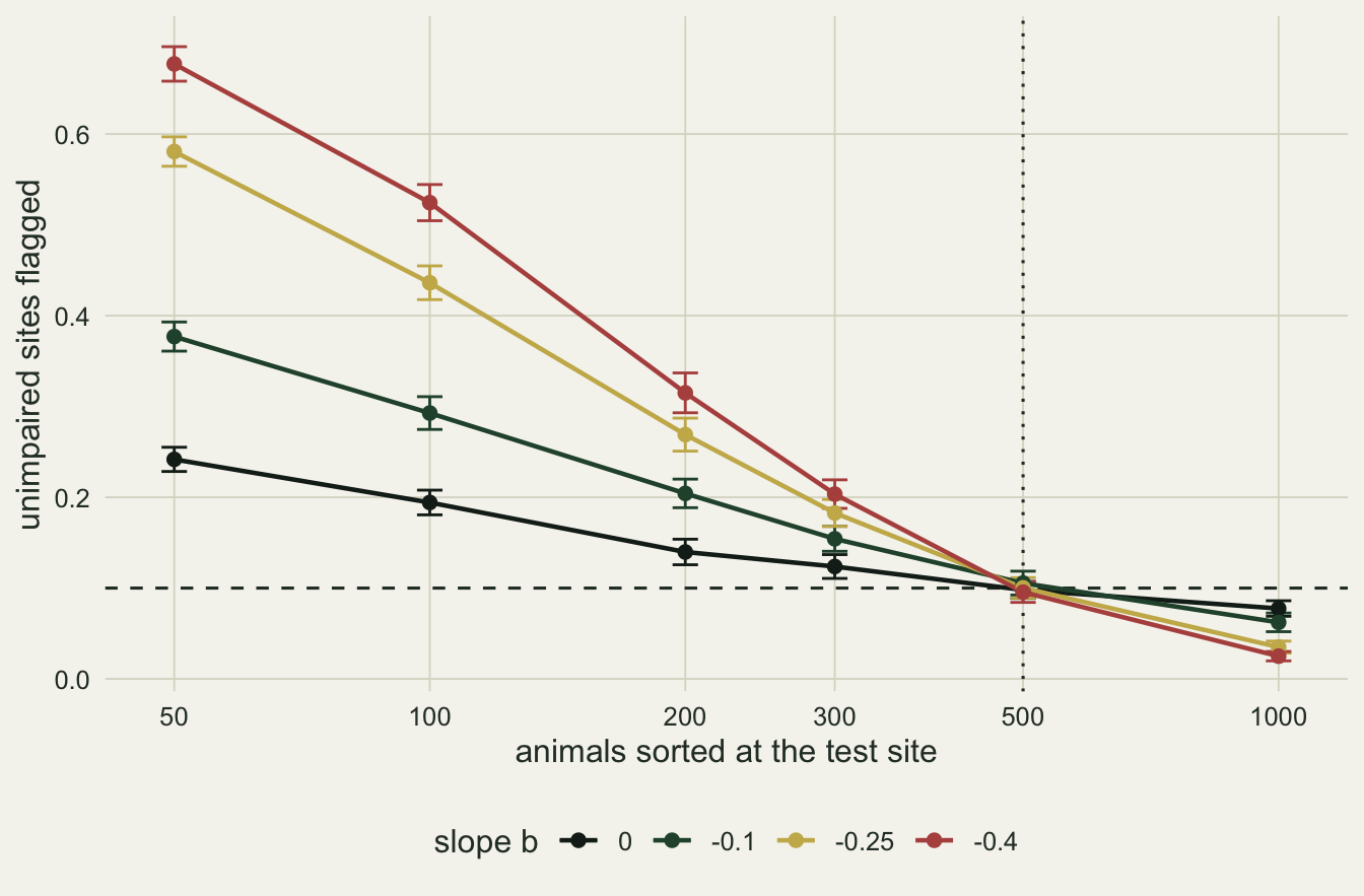
At the reference count every slope gives a rate near the intended one: 0.098, 0.105, 0.100, 0.096 for b = 0, -0.1, -0.25 and -0.4, with Monte Carlo standard errors no larger than 0.0066 at that count and no larger than 0.0110 anywhere in the table. Sort the test site to 100 animals and the rate becomes 0.436 at b = -0.25 and 0.524 at b = -0.4. At 50 animals and b = -0.25 it is 0.581. The denominator throughout is unimpaired test sites, so these are clean streams called impaired because fewer animals were picked from their trays.
The error runs the other way above the reference count. A clean site sorted to 1000 animals is flagged at 0.035 for b = -0.25, which looks like an improvement until the impaired sites are checked in the section after next.
Without any link, the spread still moves the rate
The b = 0 line in the figure is not flat either: 0.194 at 100 animals and 0.242 at 50, although the average score has no bias there. That part needs no assumption about abundance. An average over fewer families is noisier, and a percentile threshold is a statement about the spread of the reference distribution as well as its centre.
spread_tab <- do.call(rbind, lapply(c(0, -0.25), function(b) {
  r <- runs[[as.character(b)]]
  do.call(rbind, lapply(c(100, 500), function(n) {
    data.frame(slope = factor(paste("slope b =", b),
                              levels = paste("slope b =", c(0, -0.25))),
               n = paste(n, "animals"),
               aspt = r$test$aspt[, col_of(n)])
  }))
}))
thr_lines <- data.frame(
  slope = factor(paste("slope b =", c(0, -0.25)), levels = paste("slope b =", c(0, -0.25))),
  thr = sapply(c("0", "-0.25"), function(s)
    quantile(runs[[s]]$ref$aspt[, col_of(n_ref)], q_flag, names = FALSE)))
sd_of <- function(b, n) sd(runs[[as.character(b)]]$test$aspt[, col_of(n)])
sd_true0 <- sd(runs[["0"]]$test$true_aspt)ggplot(spread_tab, aes(aspt, fill = n, colour = n)) +
geom_density(alpha = 0.35, linewidth = 0.6, adjust = 1.3) +
geom_vline(data = thr_lines, aes(xintercept = thr), colour = te_rust,
linewidth = 0.8) +
facet_wrap(~ slope, nrow = 1) +
scale_fill_manual(values = c("100 animals" = te_gold, "500 animals" = te_forest),
name = NULL) +
scale_colour_manual(values = c("100 animals" = te_gold, "500 animals" = te_forest),
name = NULL) +
labs(x = "ASPT-like average score", y = "density") +
theme_datasheet() +
theme(legend.position = "bottom")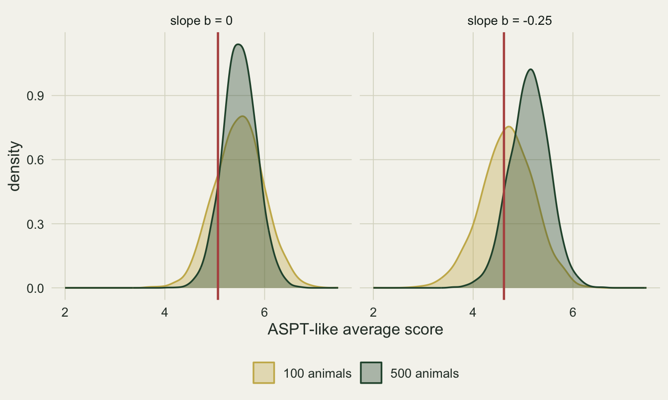
At b = 0 the two curves share a centre and differ in width: the standard deviation of the average among clean sites is 0.488 at 100 animals and 0.343 at 500; real variation among sites in which families they hold has standard deviation 0.286, 0.34 of the variance at 100 animals. The wider curve puts more mass below a threshold set on the narrower one. At b = -0.25 the curve for 100 animals is shifted to the left as well as widened, and the rate at 100 animals is 0.436 there against 0.194 at b = 0.
The same spread effect reaches the share of sensitive animals, which has no drift at all. With the threshold from references at 500 animals, clean sites sorted to 50 were flagged at 0.144, 0.106, 0.148, 0.194 for the four slopes. Three are clearly above the intended 0.10, and the b = -0.1 value is within one standard error of it; Monte Carlo standard errors are 0.0057, 0.0118, 0.0053, 0.0069. The largest rate is at b = -0.4 and is not a spread effect in the usual sense: the reference threshold there is 0.012, below one animal in 50, so a clean site sorted to 50 is flagged exactly when it holds no sensitive animal, which happened at 0.194 of them. An unbiased index is not the same thing as an effort-free threshold.
Rarefy to the smaller count, not to a blanket minimum
Both repairs put the test site and the references on the same count before comparing. The first rarefies whichever sample is larger down to the smaller count: a test site sorted to 100 is compared with references rarefied to 100, and a test site sorted to 1000 is itself rarefied to 500. That is the same as an effort-specific threshold, read from the references at the test site’s own count wherever that count does not exceed the reference count. The second rarefies every site, test and reference, to 100 animals, which is the lowest count the programme accepts; a sample sorted to 50 has no value under that rule and is left out of it. Rarefying here is one random subsample, the shorter prefix of the picked sequence.
rule_cols <- setNames(c(te_rust, te_forest, te_gold), rule_names)
rep_tab <- flag_tab[flag_tab$slope == -0.25, ]
rep_tab$rule <- factor(rep_tab$rule, levels = rule_names)
rep_tab <- rep_tab[!is.na(rep_tab$false_flag), ]
p_ff <- ggplot(rep_tab, aes(n, false_flag, colour = rule)) +
  geom_hline(yintercept = q_flag, linetype = "dashed", colour = te_body) +
  geom_line(linewidth = 0.8) + geom_point(size = 1.8) +
  scale_x_log10(breaks = n_grid) +
  scale_colour_manual(values = rule_cols, name = NULL) +
  labs(x = "animals sorted at the test site", y = "unimpaired sites flagged") +
  theme_datasheet()
p_pw <- ggplot(rep_tab, aes(n, power, colour = rule)) +
  geom_line(linewidth = 0.8) + geom_point(size = 1.8) +
  scale_x_log10(breaks = n_grid) +
  scale_y_continuous(limits = c(0, 1)) +
  scale_colour_manual(values = rule_cols, name = NULL) +
  labs(x = "animals sorted at the test site", y = "impaired sites flagged") +
  theme_datasheet()
(p_ff | p_pw) + plot_layout(guides = "collect") +
  plot_annotation(theme = theme_datasheet()) &
  theme(legend.position = "bottom",
        axis.text.x = element_text(angle = 45, hjust = 1))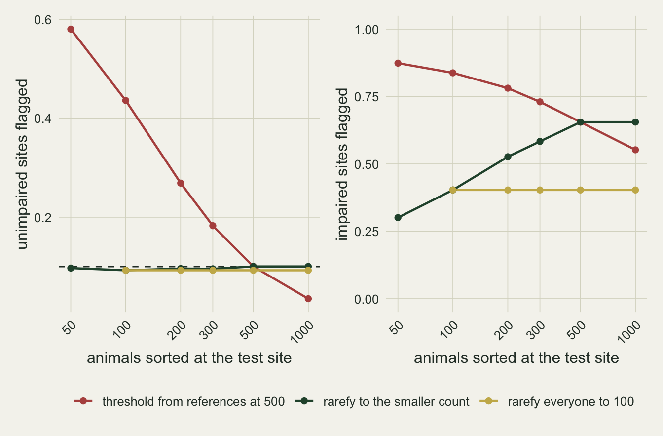
By construction both repairs compare identically distributed averages, since the clean test sites and the references come from one population and are cut to the same count, so they return the false flag rate to the intended level up to Monte Carlo error: across all slopes and counts the two rarefied rules gave rates from 0.092 to 0.111. Under the blanket rule the rate is one number per slope, repeated at every count, because every test site is cut to 100. Most of the scatter is Monte Carlo error; in the median cell 0.0015 of test sites sat exactly on the threshold. Ties matter where the threshold falls on a whole number of score units, a value an average of integer scores often takes. For b = -0.25 under the blanket rule the threshold is 4.000, 0.0145 of test sites sat exactly on it, and because a site on the threshold is not below it the rate there is 0.092 (0.107 if those sites were counted). The informative comparison is detection.
They differ in what they throw away. For b = -0.25 and a test site sorted to 500 animals, rarefying to the smaller count keeps the whole sample and detects 0.655 of impaired sites, while rarefying everyone to 100 detects 0.403. At b = 0 the same pair is 0.805 and 0.604. The blanket minimum pays for its simplicity with every sample that was sorted further than it needed to be.
The unrepaired rule looks strong at small counts, 0.838 of impaired sites flagged at 100 animals, but it flags 0.436 of clean ones at the same count, so that detection rate is not a property of the index. Above the reference count it errs the other way, with fewer false flags and less detection: at 1000 animals it detects 0.552 of impaired sites, against 0.655 for the same site rarefied to 500.
What to report
Report the number of animals sorted for every sample, next to the index, and the count the references were sorted to. Without both a reader cannot tell whether a low average score at a site is a low score or a short sort.
Compare a test site with references at the same count. Where the programme keeps the reference trays or their full picked lists, rarefy the larger of the two samples to the smaller count, which here held the false flag rate and kept the detection rate of the full sample wherever the test site was sorted no further than the references. Rarefying every sample to the lowest count in the programme also held the false flag rate and gave up detection at every site sorted further, from 0.655 to 0.403 at 500 animals for b = -0.25.
Check the assumption in the data before trusting a flat average. If the reference samples record counts per family, a regression of log count on tolerance score across the families recorded gives a rough estimate of b for that programme (rough, because families missed by the sort have no count), and an ASPT computed on successive rarefied counts of a few large reference samples shows whether the average drifts. A drift of 0.44 score units between 100 and 500 animals, on top of the wider spread at 100 animals, moved the false flag rate here from 0.100 to 0.436, against 0.194 from the spread alone at b = 0.
Even with no link at all, state the spread; this result, unlike the drift, needs no assumption about abundance and tolerance. A threshold that is a percentile of references belongs to the count those references were sorted to, and at b = 0 a 100-animal test site was flagged at 0.194 against a 500-animal reference set.
Honest limits
The abundance-tolerance slope is assumed, not estimated from any real programme. In European kick samples some tolerant families (chironomids, oligochaetes) are routinely the most numerous, but so are some mid-scoring ones such as gammarids and baetids, and sensitive stoneflies and heptageniids can be abundant at clean upland sites. A real pool will not have a single log-linear slope, and the sign may change between river types. The post shows what follows if the link is negative; it does not show that it is. The one test of effort on ASPT itself cited here points the other way at UK sample sizes: Armitage and colleagues found that replicate samples changed ASPT little. That fits a weak link, or a negative one whose drift has levelled off by the counts in a whole-sorted kick sample; it gives no support to a slope as steep as -0.25 at a 100-animal count. Every departure from the b = 0 line rests on that slope.
Sorting is simulated as random picks with replacement from an infinite site population. Real sorting draws from a finite tray without replacement, and laboratory pickers do not pick at random: large and conspicuous animals tend to be picked first, which is a second source of family order that could push the drift either way. Fixed-count subsampling by grid cells, the procedure Barbour and Gerritsen describe, is closer to random than hand picking but still spatially clumped within the tray. Fixed-count picking is standard in North American programmes and in some European ones, where the German AQEM work of Lorenz and colleagues tested subsamples of 100 to 700 individuals, whereas UK BMWP and RIVPACS samples are normally sorted whole, so there the effort difference lies in the kick sample itself rather than in the laboratory count.
The scores are a stylised 1 to 10 pool with seven families per score, and presence is independent among families. Real BMWP scores are unevenly spread over families, real communities have correlated occurrences, and the published BMWP and ASPT carry extra rules (family groupings, scores for taxa that share a family) that are not modelled.
The rarefied rules use one random subsample. Averaging over many subsamples, or computing the expected family list at the smaller count from the full counts, would reduce the noise that rarefying adds and raise the detection rates of both repairs somewhat; it was not measured. Rarefying the test site down when it was sorted beyond the reference count also discards information that an effort-specific threshold built from larger reference sorts would keep.
Impairment is one pattern, halved presence of families scoring 7 to 10, at one strength. Detection rates depend on both, and on b, and the power comparisons quoted belong to this design. Modern assessment schemes predict the expected fauna at each site from its environment, as RIVPACS does in Clarke and colleagues, and compare observed with expected rather than with a flat percentile; the effort mismatch applies to that ratio too, because the expected list is also calibrated on samples processed a particular way, but that version was not simulated.
References
Armitage PD, Moss D, Wright JF, Furse MT 1983 Water Research 17(3):333-347 (10.1016/0043-1354(83)90188-4)
Vinson MR, Hawkins CP 1996 Journal of the North American Benthological Society 15(3):392-399 (10.2307/1467286)
Barbour MT, Gerritsen J 1996 Journal of the North American Benthological Society 15(3):386-391 (10.2307/1467285)
Lorenz AW, Kirchner L, Hering D 2004 Hydrobiologia 516(1-3):299-312 (10.1023/B:HYDR.0000025272.05793.00)
Clarke RT, Wright JF, Furse MT 2003 Ecological Modelling 160(3):219-233 (10.1016/S0304-3800(02)00255-7)