---
title: "Bayesian logistic regression under separation"
description: "When a predictor perfectly separates presence from absence the logistic MLE diverges. A weakly-informative Cauchy prior fixes it, coded from scratch in base R."
date: "2026-07-15 11:00"
categories: [R, Bayesian statistics, MCMC, logistic regression, ecology tutorial]
image: thumbnail.png
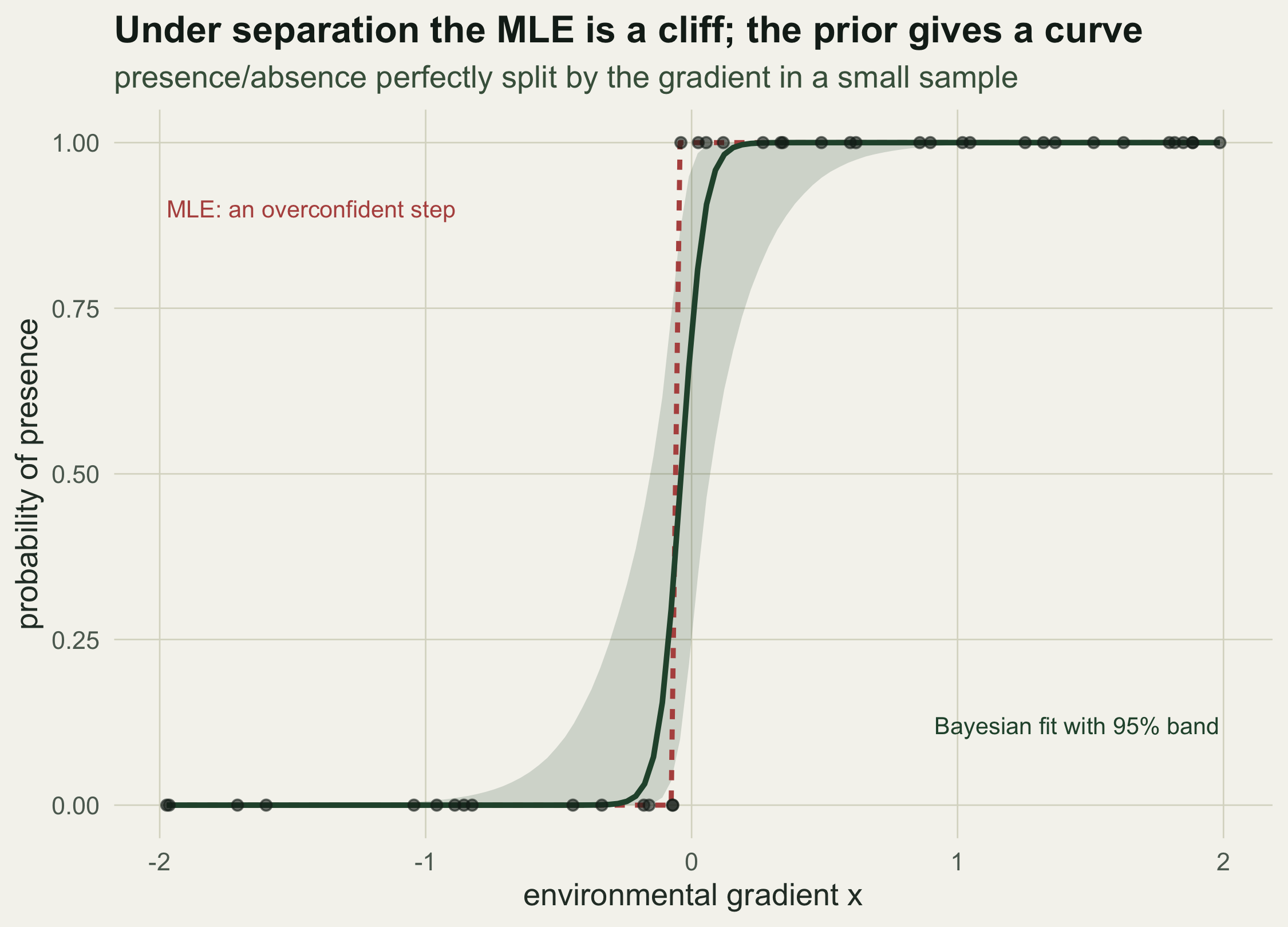
image-alt: "Fitted probability of presence against an environmental gradient; the maximum-likelihood fit is a vertical cliff pinned at zero and one, while the Bayesian fit is a smooth curve with a wide credible band in the data gap."
---
```{r}
#| label: setup
#| include: false
knitr::opts_chunk$set(message = FALSE, warning = FALSE,
fig.width = 7.5, fig.height = 5.4, dpi = 150)
library(ggplot2)
te <- list(ink="#16241d", body="#2c3a31", forest="#275139", label="#46604a",
sage="#93a87f", paper="#f5f4ee", line="#dad9ca", faint="#5d6b61",
gold="#cda23f", mown="#2f8f63", terra="#b5534e")
theme_te <- function(base_size = 13) {
theme_minimal(base_size = base_size) +
theme(plot.background = element_rect(fill = te$paper, colour = NA),
panel.background = element_rect(fill = te$paper, colour = NA),
panel.grid.major = element_line(colour = te$line, linewidth = 0.3),
panel.grid.minor = element_blank(),
axis.text = element_text(colour = te$faint),
axis.title = element_text(colour = te$body),
plot.title = element_text(colour = te$ink, face = "bold"),
plot.subtitle = element_text(colour = te$label),
legend.text = element_text(colour = te$body),
plot.caption = element_text(colour = te$faint, size = base_size * 0.75))
}
```
[Logistic regression](../logistic-regression-presence-absence/) is the default
tool for presence and absence, and its default fit is maximum likelihood through
`glm`. That fit quietly assumes the data actually pin the coefficients down. When a
predictor separates the two classes too well, so that presence is recorded at
every site above some value on a gradient and at none below it, the assumption
fails: the slope runs off towards infinity, `glm` returns an enormous estimate
with an even larger standard error, and every fitted probability collapses to zero
or one. This is complete separation (Albert and Anderson 1984), and it is common
in small ecological samples on strong gradients. A weakly-informative prior turns
the broken fit into a sensible one, and this post codes the whole thing from
scratch in base R.
## A perfectly separated survey
We take forty sites along an environmental gradient `x`, with presence recorded at
every site above a threshold and absence at every site below it. Nothing overlaps.
```{r}
#| label: data
set.seed(4)
n <- 40
x <- sort(runif(n, -2, 2))          # a standardised gradient, e.g. temperature
x_split <- mean(x[15:16])
y <- as.integer(x > x_split)        # presence above the threshold, absence below
c(presences = sum(y), absences = sum(1 - y))
paste(y, collapse = "")
```
## The maximum-likelihood fit falls apart
```{r}
#| label: glm
g  <- suppressWarnings(glm(y ~ x, family = binomial))
cf <- summary(g)$coefficients
round(cf, 2)
```
The slope estimate is `r format(round(cf["x", "Estimate"]), big.mark = " ")`
with a standard error of
`r format(round(cf["x", "Std. Error"]), big.mark = " ")`: the point estimate is
meaningless and the standard error announces as much. The algorithm did not
converge (`glm` stops at its iteration limit with `converged` equal to
`r g$converged`), every fitted probability has been pushed to
`r round(min(fitted(g)))` or `r round(max(fitted(g)))`, and the Wald 95% interval
for the slope runs from about
`r format(round(cf["x","Estimate"] - 1.96*cf["x","Std. Error"]), big.mark=" ")` to
`r format(round(cf["x","Estimate"] + 1.96*cf["x","Std. Error"]), big.mark=" ")`.
None of this is a numerical glitch to be patched with more iterations. The
likelihood simply keeps increasing as the slope grows, so it has no maximum, and
the estimate that maximises it does not exist.
## A weakly-informative prior
The fix is to say something mild and defensible before seeing the data: that a
one-unit change in a predictor is unlikely to multiply the odds by an astronomical
factor. Gelman (2008) turns this into a default: scale each non-binary predictor to
a standard deviation of 0.5, then put an independent Cauchy prior with centre 0 and
scale 2.5 on each slope, and a wider Cauchy on the intercept. The Cauchy has heavy
tails, so it barely touches the estimate when the data are informative, but it is
enough to give the posterior a finite peak when they are not. We sample it with a
plain random-walk [Metropolis sampler](../metropolis-hastings-from-scratch/).
```{r}
#| label: bayes
xs <- (x - mean(x)) / (2 * sd(x))                 # scale to SD 0.5 (Gelman 2008)
logpost <- function(b) {
  eta <- b[1] + b[2] * xs
  sum(dbinom(y, 1, plogis(eta), log = TRUE)) +
    dcauchy(b[1], 0, 10, log = TRUE) + dcauchy(b[2], 0, 2.5, log = TRUE)
}
metropolis <- function(iter = 60000, warm = 10000, step = c(0.6, 0.7), seed = 1) {
  set.seed(seed)
  b <- c(0, 0); lp <- logpost(b); out <- matrix(NA_real_, iter, 2); acc <- 0
  for (t in seq_len(iter)) {
    prop <- b + rnorm(2, 0, step)
    lpp  <- logpost(prop)
    if (log(runif(1)) < lpp - lp) { b <- prop; lp <- lpp; acc <- acc + 1 }
    out[t, ] <- b
  }
  list(draws = out[(warm + 1):iter, ], acc = acc / iter)
}
fit    <- metropolis(seed = 21)
draws  <- fit$draws
b1_org <- draws[, 2] / (2 * sd(x))                # slope back on the x scale
```
The chain accepts `r sprintf("%.0f", 100 * fit$acc)`% of proposals. On the original
gradient scale the posterior median slope is
`r sprintf("%.1f", median(b1_org))` with a 95% credible interval of
`r sprintf("[%.1f, %.1f]", quantile(b1_org, .025), quantile(b1_org, .975))`. That
interval is wide and its upper end is soft, which is the honest situation: the data
fix how fast presence rises but put no ceiling on it, so the slope is large and
uncertain rather than infinite. The quantity to report is not the slope but the
fitted probability, where the uncertainty lands where it should.
```{r}
#| label: fig-curves
#| fig-cap: "Fitted probability of presence along the gradient. The maximum-likelihood fit (dashed) is a vertical cliff, pinned at zero below the threshold and one above it with no acknowledged uncertainty. The Bayesian posterior median (solid) is a smooth curve whose 95% credible band widens across the gap between the last absence and the first presence, exactly where the data are silent."
#| fig-alt: "Presence-absence points at zero and one along the x axis. A dashed red maximum-likelihood curve rises vertically at the threshold. A solid green Bayesian curve rises gradually through the same region, surrounded by a shaded band that is widest in the gap between the classes."
xg  <- seq(min(x), max(x), length.out = 120)
xgs <- (xg - mean(x)) / (2 * sd(x))
pmat <- plogis(outer(draws[, 1], rep(1, length(xg))) + outer(draws[, 2], xgs))
bfit <- data.frame(x = xg, med = apply(pmat, 2, median),
                   lo = apply(pmat, 2, quantile, .025), hi = apply(pmat, 2, quantile, .975))
gfit <- data.frame(x = xg, p = predict(g, data.frame(x = xg), type = "response"))
ggplot() +
  geom_ribbon(data = bfit, aes(x, ymin = lo, ymax = hi), fill = te$forest, alpha = 0.18) +
  geom_line(data = gfit, aes(x, p), colour = te$terra, linewidth = 1, linetype = "22") +
  geom_line(data = bfit, aes(x, med), colour = te$forest, linewidth = 1.1) +
  geom_point(data = data.frame(x = x, y = y), aes(x, y), colour = te$ink, alpha = 0.6, size = 1.8) +
  annotate("text", x = min(x), y = 0.9, hjust = 0, size = 3.5, colour = te$terra,
           label = "MLE: an overconfident step") +
  annotate("text", x = max(x), y = 0.12, hjust = 1, size = 3.5, colour = te$forest,
           label = "Bayesian fit with 95% band") +
  labs(x = "environmental gradient x", y = "probability of presence",
       title = "Under separation the MLE is a cliff; the prior gives a curve",
       subtitle = "presence/absence perfectly split by the gradient in a small sample") +
  theme_te()
```
```{r}
#| label: gap
xq  <- c(x[15], x_split, x[16])
qs  <- (xq - mean(x)) / (2 * sd(x))
pm  <- plogis(outer(draws[, 1], rep(1, 3)) + outer(draws[, 2], qs))
gap <- round(apply(pm, 2, quantile, c(.025, .5, .975)), 2)
colnames(gap) <- c("last absence", "gap centre", "first presence"); gap
```
The gap between the last absence and the first presence spans only
`r sprintf("%.2f", x[16] - x[15])` units of the gradient. Across it the
maximum-likelihood curve jumps from `r round(predict(g, data.frame(x = x[15]), type="response"))`
to `r round(predict(g, data.frame(x = x[16]), type="response"))`, a near-certain
verdict either side of a hair-thin line. The Bayesian fit, at the centre of that
gap, puts the probability of presence at `r sprintf("%.2f", gap[2, "gap centre"])`
with a 95% band from `r sprintf("%.2f", gap[1, "gap centre"])` to
`r sprintf("%.2f", gap[3, "gap centre"])`: it admits that it does not know, which
is correct.
## Why the prior works
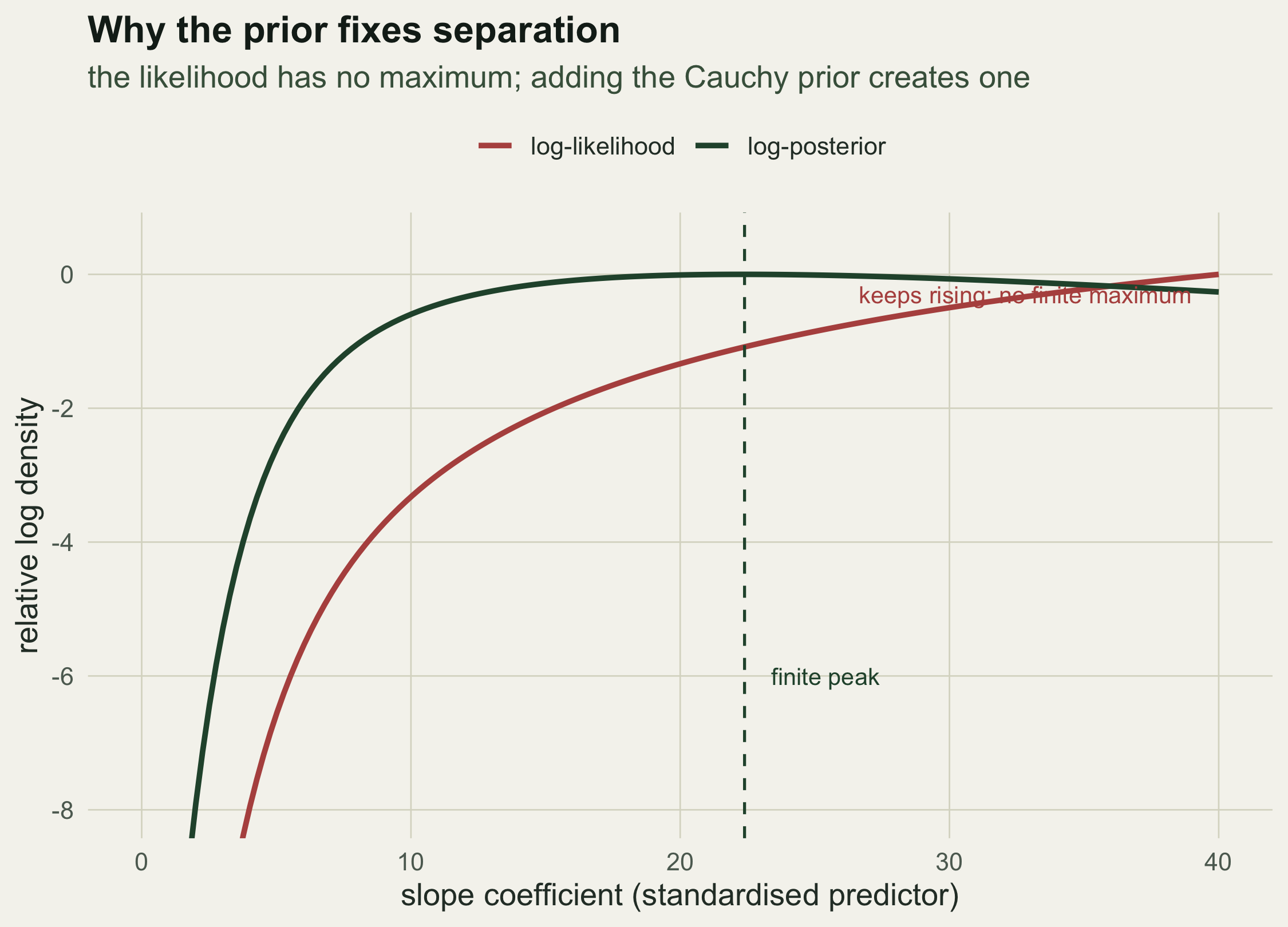
The mechanism is visible in the likelihood itself. Profiling out the intercept and
tracing the log-likelihood as the slope grows, it climbs and flattens but never
turns over, so its maximum sits at infinity. Adding the log prior tilts the curve
just enough to produce a finite peak.
```{r}
#| label: profile
loglik <- function(b) sum(dbinom(y, 1, plogis(b[1] + b[2] * xs), log = TRUE))
b1grid <- seq(0, 40, length.out = 160)
prof <- t(sapply(b1grid, function(b1) c(
  ll = -optimize(function(b0) -loglik(c(b0, b1)),  c(-30, 30))$objective,
  lp = -optimize(function(b0) -logpost(c(b0, b1)), c(-30, 30))$objective)))
ll_rising   <- which.max(prof[, "ll"]) == length(b1grid)
b1_hat_post <- b1grid[which.max(prof[, "lp"])]
c(likelihood_still_rising_at_edge = ll_rising, posterior_peak = round(b1_hat_post, 1))
```
The log-likelihood is
`r if (ll_rising) "still rising at the edge of the grid" else "turning over"`,
confirming that no finite slope maximises it, while the log-posterior peaks near a
slope of `r round(b1_hat_post, 1)` on the standardised scale. The prior supplies
the curvature that the data do not.
```{r}
#| label: fig-profile
#| fig-cap: "Profile log-likelihood and log-posterior for the slope, each shown relative to its own maximum. The log-likelihood rises without bound, so the maximum-likelihood estimate does not exist; the Cauchy prior adds enough curvature to give the log-posterior a finite peak, marked by the dashed line."
#| fig-alt: "Two curves against the slope coefficient. The red log-likelihood curve rises and flattens towards zero but never peaks. The green log-posterior curve rises to a clear maximum around a slope of 22 and then falls."
dfp <- rbind(
  data.frame(b1 = b1grid, val = prof[, "ll"] - max(prof[, "ll"]), curve = "log-likelihood"),
  data.frame(b1 = b1grid, val = prof[, "lp"] - max(prof[, "lp"]), curve = "log-posterior"))
ggplot(dfp, aes(b1, val, colour = curve)) +
  geom_line(linewidth = 1.1) +
  geom_vline(xintercept = b1_hat_post, linetype = "dashed", colour = te$forest) +
  scale_colour_manual(values = c("log-likelihood" = te$terra, "log-posterior" = te$forest), name = NULL) +
  coord_cartesian(ylim = c(-8, 0.5)) +
  annotate("text", x = 39, y = -0.3, hjust = 1, size = 3.5, colour = te$terra,
           label = "keeps rising: no finite maximum") +
  annotate("text", x = b1_hat_post + 1, y = -6, hjust = 0, size = 3.5, colour = te$forest,
           label = "finite peak") +
  labs(x = "slope coefficient (standardised predictor)", y = "relative log density",
       title = "Why the prior fixes separation",
       subtitle = "the likelihood has no maximum; adding the Cauchy prior creates one") +
  theme_te() + theme(legend.position = "top")
```
## Other ways out, and what to report
The frequentist counterpart to the prior is a penalty. Firth (1993) reduces the
bias of maximum likelihood with a penalty equal to the Jeffreys prior, and as a
by-product that penalty also gives finite estimates under separation; it is what
the `logistf` package does. Penalised likelihood and a weakly-informative prior are
two views of the same repair, one adding a penalty to the log-likelihood and the
other adding a log prior, and here they land in the same place. The Bayesian route
has the edge that it hands back a full posterior, so the credible band on the
fitted curve comes for free rather than needing a separate approximation.
Whichever repair you use, separation is worth reading as a message rather than an
error. It says the sample does not contain the information to pin one parameter, so
any single number for that parameter is an artefact of the fitting method. The
[Wald interval](../standard-errors-confidence-intervals/) that `glm` prints under
separation is not a wide-but-honest interval; it is meaningless, built from a
standard error that does not describe anything. The credible interval, and the
fitted-probability band that widens exactly where the classes fail to overlap, is
the honest replacement, and it is the thing to put in the paper.
## References
- Albert A, Anderson JA 1984 Biometrika 71(1):1-10 (10.1093/biomet/71.1.1)
- Firth D 1993 Biometrika 80(1):27-38 (10.1093/biomet/80.1.27)
- Gelman A, Jakulin A, Pittau MG, Su Y-S 2008 Annals of Applied Statistics 2(4):1360-1383 (10.1214/08-AOAS191)
- Gelman A, Hill J 2007 Data Analysis Using Regression and Multilevel/Hierarchical Models (ISBN 978-0-521-68689-1)
- McElreath R 2020 Statistical Rethinking, 2nd edn (ISBN 978-0-367-13991-9)
## Related tutorials
- [Logistic regression for presence-absence data](../logistic-regression-presence-absence/)
- [Standard errors and confidence intervals](../standard-errors-confidence-intervals/)
- [Metropolis-Hastings from scratch](../metropolis-hastings-from-scratch/)
- [Collinearity and the variance inflation factor](../collinearity-and-vif/)