Validating a step selection model

Used-habitat calibration plots from scratch: simulate used locations from a fitted step selection model and check if it reproduces the chosen habitat.

A fitted step selection model can reproduce the used-against-available contrast it was trained on and still be wrong about the habitat. The coefficients might be significant, the likelihood healthy, and the functional form quietly mistaken. The check that catches this asks a different question: if we take the fitted model and simulate where the animal would go, does the habitat at those simulated steps match the habitat at the real ones? That is a used-habitat calibration plot (Fieberg and colleagues 2018), and it closes this thread the same way pseudo-residuals closed the movement HMM and innovations closed the state-space model.

An animal that likes the middle

We give the animal two covariates. It selects linearly for a resource, as before, but for a second covariate, cover, it prefers intermediate values and avoids both extremes. That is a quadratic on cover with a negative squared term, the kind of hump a linear covariate cannot represent.

library(ggplot2)
library(grid)

res_raw <- function(x, y)
  1.4 * exp(-((x - 38)^2 + (y - 62)^2) / (2 * 24^2)) +
  1.1 * exp(-((x - 68)^2 + (y - 40)^2) / (2 * 26^2)) -
  0.00030 * ((x - 50)^2 + (y - 50)^2)
cov_raw <- function(x, y) sin(x / 15) * cos(y / 13) + 0.6 * sin((x + y) / 19)
gx <- seq(0, 100, length.out = 130); gd <- expand.grid(x = gx, y = gx)
mr <- mean(res_raw(gd$x, gd$y)); sr <- sd(res_raw(gd$x, gd$y))
mc <- mean(cov_raw(gd$x, gd$y)); sc <- sd(cov_raw(gd$x, gd$y))
resource <- function(x, y) (res_raw(x, y) - mr) / sr
cover    <- function(x, y) (cov_raw(x, y) - mc) / sc

rvm <- function(n, mu, kappa) {
  out <- numeric(n); a <- 1 + sqrt(1 + 4 * kappa^2)
  b <- (a - sqrt(2 * a)) / (2 * kappa); r <- (1 + b^2) / (2 * b)
  for (i in seq_len(n)) {
    repeat {
      u1 <- runif(1); u2 <- runif(1); u3 <- runif(1)
      z <- cos(pi * u1); f <- (1 + r * z) / (r + z); cc <- kappa * (r - f)
      if (cc * (2 - cc) - u2 > 0 || log(cc / u2) + 1 - cc >= 0) break
    }
    out[i] <- sign(u3 - 0.5) * acos(f) + mu
  }
  ((out + pi) %% (2 * pi)) - pi
}

b_res <- 0.8; b_cov <- 0.0; b_cov2 <- -0.7
k_move <- 2.0; th_move <- 5.5; kap_move <- 0.9
n <- 1200; M <- 300
set.seed(2718)
pos <- matrix(NA_real_, n + 1, 2); pos[1, ] <- c(45, 50)
heading <- numeric(n + 1); heading[1] <- runif(1, -pi, pi)
for (i in 1:n) {
  L <- rgamma(M, shape = k_move, scale = th_move); a <- rvm(M, 0, kap_move)
  ang <- heading[i] + a
  ex <- pos[i, 1] + L * cos(ang); ey <- pos[i, 2] + L * sin(ang)
  cv <- cover(ex, ey)
  w <- exp(b_res * resource(ex, ey) + b_cov * cv + b_cov2 * cv^2)
  j <- sample.int(M, 1, prob = w)
  pos[i + 1, ] <- c(ex[j], ey[j]); heading[i + 1] <- ang[j]
}
dx <- diff(pos[, 1]); dy <- diff(pos[, 2])
obs_l <- sqrt(dx^2 + dy^2); bearing <- atan2(dy, dx)
obs_turn <- ((diff(bearing) + pi) %% (2 * pi)) - pi
m1 <- mean(obs_l); v1 <- var(obs_l); k0 <- m1^2 / v1; th0 <- v1 / m1
Cc <- mean(cos(obs_turn)); Ss <- mean(sin(obs_turn)); Rbar <- sqrt(Cc^2 + Ss^2); mu0 <- atan2(Ss, Cc)
kap0 <- if (Rbar < 0.85) -0.4 + 1.39 * Rbar + 0.43 / (1 - Rbar) else 1 / (Rbar^3 - 4 * Rbar^2 + 3 * Rbar)

We build strata as usual, one used step and fifteen available steps drawn from the tentative kernel, and store the resource and cover at every point.

K <- 15; set.seed(11223)
use_idx <- 2:n; n_str <- length(use_idx); Sp <- K + 1
res_m <- cov_m <- matrix(NA_real_, Sp, n_str)     # row 1 = used, rows 2..Sp = available
for (s in seq_along(use_idx)) {
  i <- use_idx[s]
  res_m[1, s] <- resource(pos[i + 1, 1], pos[i + 1, 2])
  cov_m[1, s] <- cover(pos[i + 1, 1], pos[i + 1, 2])
  Ls <- rgamma(K, shape = k0, scale = th0); As <- rvm(K, mu0, kap0)
  ang <- heading[i] + As
  ax <- pos[i, 1] + Ls * cos(ang); ay <- pos[i, 2] + Ls * sin(ang)
  res_m[2:Sp, s] <- resource(ax, ay); cov_m[2:Sp, s] <- cover(ax, ay)
}

Two models, one of them wrong

We fit the correct model, with resource, cover and cover squared, and a tempting shortcut that keeps cover linear. Both use the conditional logistic likelihood built earlier.

fit_clogit <- function(mats) {
  p <- length(mats)
  nll <- function(b) {
    eta <- matrix(0, Sp, n_str)
    for (j in 1:p) eta <- eta + b[j] * mats[[j]]
    -sum(eta[1, ] - log(colSums(exp(eta))))
  }
  o <- optim(rep(0, p), nll, method = "BFGS", hessian = TRUE, control = list(reltol = 1e-10))
  list(b = o$par, V = solve(o$hessian))
}
fit_full <- fit_clogit(list(res_m, cov_m, cov_m^2))
fit_lin  <- fit_clogit(list(res_m, cov_m))
se_lin <- sqrt(diag(fit_lin$V))

The full model recovers the truth: resource 0.77, cover -0.03 and cover squared -0.68, against true values of 0.8, 0 and -0.7. The linear model reports a cover coefficient of 0.11 with a standard error of 0.054, a z of 1.99 that scrapes past the usual threshold. Read on its own that number invites a story about a weak preference for higher cover. The story is wrong: the animal likes the middle, and a straight line has no middle. Nothing in the coefficient table says so.

Simulating used habitat from the fit

The calibration plot makes the model predict, then checks the prediction. For each of many draws we take a parameter vector from the model’s sampling distribution, use it to weight the available steps in every stratum, and sample one step per stratum as the model says the animal would choose. The cover values at those simulated steps give one predicted used-habitat distribution; the spread across draws gives an envelope. If the model is right, the cover the animal really used lies inside it.

uhc_env <- function(fit, mats, focal, grid, B = 300) {
  p <- length(mats); Lc <- chol(fit$V)
  dens <- matrix(NA_real_, length(grid), B)
  for (bb in 1:B) {
    beta <- as.vector(fit$b + t(Lc) %*% rnorm(p))     # draw from the sampling distribution
    eta <- matrix(0, Sp, n_str)
    for (j in 1:p) eta <- eta + beta[j] * mats[[j]]
    P <- exp(eta); P <- sweep(P, 2, colSums(P), "/")
    cumP <- apply(P, 2, cumsum)
    u <- runif(n_str)
    idx <- colSums(sweep(cumP, 2, u, "<")) + 1        # one sampled step per stratum
    picked <- focal[cbind(idx, seq_len(n_str))]
    dens[, bb] <- density(picked, from = min(grid), to = max(grid),
                          n = length(grid), bw = 0.25)$y
  }
  data.frame(x = grid, lo = apply(dens, 1, quantile, 0.025),
             hi = apply(dens, 1, quantile, 0.975))
}

grid <- seq(-2.6, 2.6, length.out = 200)
obs_dens <- density(cov_m[1, ], from = min(grid), to = max(grid), n = length(grid), bw = 0.25)
env_full <- uhc_env(fit_full, list(res_m, cov_m, cov_m^2), cov_m, grid)
env_lin  <- uhc_env(fit_lin,  list(res_m, cov_m),          cov_m, grid)
frac_out <- function(env) 100 * mean(obs_dens$y < env$lo - 1e-8 | obs_dens$y > env$hi + 1e-8)

The verdict is stark. Under the full model, the observed used-cover curve sits entirely inside the envelope, with 0 per cent of it outside. Under the linear model, 86 per cent falls outside: the animal concentrated its steps at intermediate cover, with a used spread of 0.61 against an available spread of 0.79, and the linear model, seeing no line that fits, predicts almost no concentration at all.

mk <- function(env, ttl) {
  ggplot() +
    geom_ribbon(data = env, aes(x, ymin = lo, ymax = hi), fill = "#93a87f", alpha = 0.45) +
    geom_line(data = data.frame(x = obs_dens$x, y = obs_dens$y), aes(x, y),
              colour = "#b5534e", linewidth = 0.8) +
    labs(x = "cover at used step", y = "density", title = ttl) +
    theme_minimal(base_size = 11) +
    theme(panel.grid.minor = element_blank(), plot.title = element_text(size = 10, colour = "#46604a"))
}
grid.newpage(); pushViewport(viewport(layout = grid.layout(1, 2)))
print(mk(env_full, "Full model (resource + cover + cover^2)"), vp = viewport(layout.pos.col = 1))
print(mk(env_lin, "Linear model (resource + cover)"), vp = viewport(layout.pos.col = 2))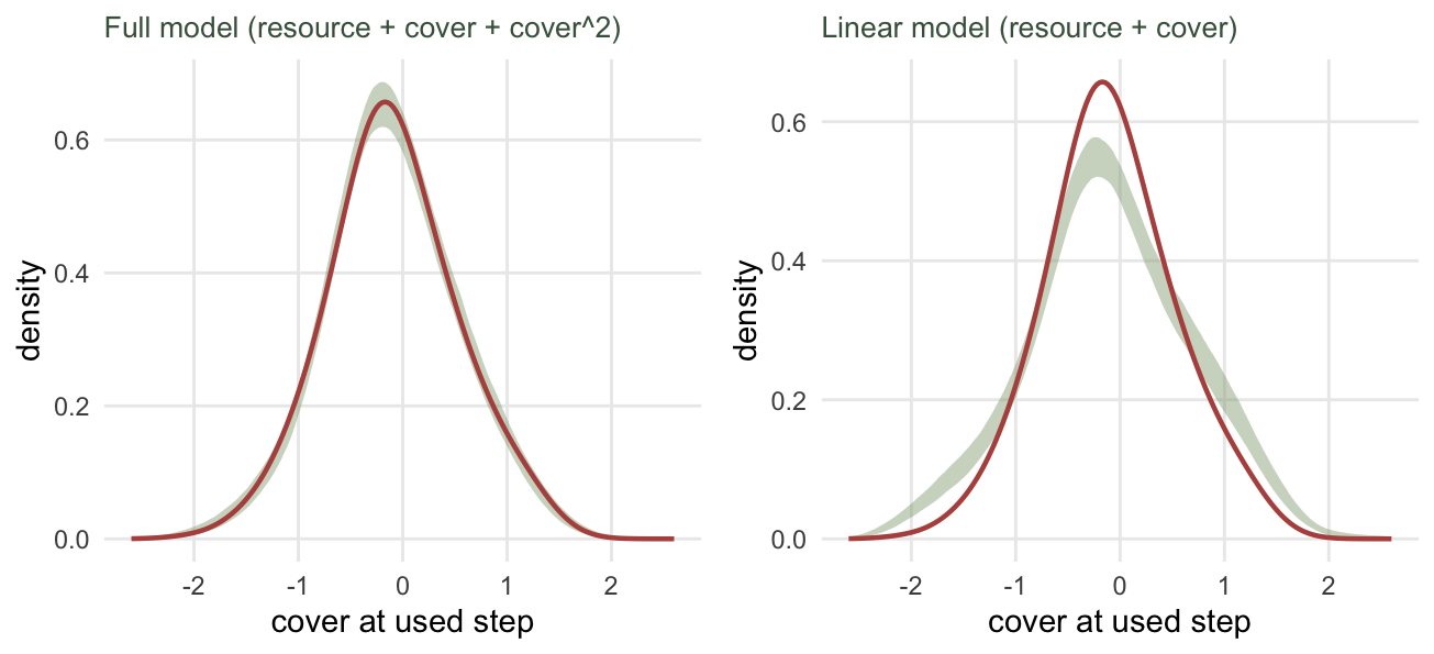

Figure 1: Used-habitat calibration for cover. The observed distribution of cover at used steps (red) is compared with the envelope simulated from each fitted model (green). The full model contains the observed curve; the linear model does not, because it cannot represent a preference for intermediate cover.

What the plot is telling you

The failure is not a mystery once you plot what each model believes about cover. The true preference is a hump; the full fit reproduces it; the linear fit draws the only shape it can, a gentle slope that says next to nothing.

cc <- seq(-2.4, 2.4, length.out = 200)
rss_df <- rbind(
  data.frame(model = "true", cover = cc, y = b_cov * cc + b_cov2 * cc^2),
  data.frame(model = "full fit", cover = cc, y = fit_full$b[2] * cc + fit_full$b[3] * cc^2),
  data.frame(model = "linear fit", cover = cc, y = fit_lin$b[2] * cc))
rss_df$model <- factor(rss_df$model, levels = c("true", "full fit", "linear fit"))
ggplot(rss_df, aes(cover, y, colour = model, linetype = model)) +
  geom_hline(yintercept = 0, colour = "#dad9ca") +
  geom_line(linewidth = 0.8) +
  scale_colour_manual(values = c("true" = "#16241d", "full fit" = "#275139", "linear fit" = "#b5534e")) +
  scale_linetype_manual(values = c("true" = "22", "full fit" = "solid", "linear fit" = "solid")) +
  labs(x = "cover (standardised)", y = "log relative selection", colour = NULL, linetype = NULL,
       title = "A straight line cannot capture a peak") +
  theme_minimal(base_size = 11) +
  theme(panel.grid.minor = element_blank(), legend.position = c(0.5, 0.2),
        legend.direction = "horizontal",
        legend.background = element_rect(fill = "#ffffff", colour = NA),
        plot.title = element_text(size = 10, colour = "#46604a"))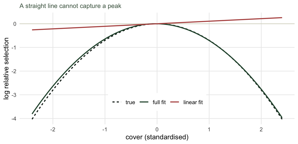

Figure 2: Fitted log relative selection against cover. The true preference for intermediate cover (dashed) is a hump that the full model recovers and the linear model cannot approach.

Two things are worth keeping. First, the plot is covariate by covariate: the resource here is truly linear and both models pass its calibration, so the failure points a finger straight at cover, not at the model in general. That is how a calibration plot turns a vague sense of misfit into a specific covariate to reconsider. Second, the honest version of this check splits the track into training and testing halves and validates on the half the model never saw, which also guards against a flexible model fitting noise; the in-sample version here is enough to expose a missing functional form. With that, the arc from a basic step selection function through the integrated model and its availability sampling to a fitted model you have actually checked is complete.

References

Fieberg J, Forester JD, Street GM, Johnson DH, ArchMiller AA, Matthiopoulos J 2018. Ecography 41(5):737-752 (10.1111/ecog.03123).

Avgar T, Potts JR, Lewis MA, Boyce MS 2016. Methods in Ecology and Evolution 7(5):619-630 (10.1111/2041-210X.12528).

Fieberg J, Signer J, Smith B, Avgar T 2021. Journal of Animal Ecology 90(5):1027-1043 (10.1111/1365-2656.13441).

Forester JD, Im HK, Rathouz PJ 2009. Ecology 90(12):3554-3565 (10.1890/08-0874.1).

Boyce MS, Vernier PR, Nielsen SE, Schmiegelow FKA 2002. Ecological Modelling 157(2-3):281-300 (10.1016/S0304-3800(02)00200-4).

Signer J, Fieberg J, Avgar T 2019. Ecology and Evolution 9(2):880-890 (10.1002/ece3.4823).

Related tutorials

• Integrated step selection analysis
• Step selection functions
• Availability sampling for step selection
• Checking a state-space movement model