library(ggplot2)
library(dplyr)
library(tidyr)

pal <- list(ink = "#16241d", body = "#2c3a31", forest = "#275139", label = "#46604a",
            sage = "#93a87f", paper = "#f5f4ee", line = "#dad9ca", faint = "#5d6b61")
state_cols <- c(Encamped = "#cda23f", Transiting = "#275139")
theme_te <- function(base_size = 12) {
  theme_minimal(base_size = base_size) +
    theme(plot.background = element_rect(fill = pal$paper, colour = NA),
          panel.background = element_rect(fill = pal$paper, colour = NA),
          panel.grid.major = element_line(colour = pal$line, linewidth = 0.3),
          panel.grid.minor = element_blank(),
          axis.text = element_text(colour = pal$faint), axis.title = element_text(colour = pal$body),
          plot.title = element_text(colour = pal$ink, face = "bold"),
          plot.subtitle = element_text(colour = pal$label),
          strip.text = element_text(colour = pal$ink, face = "bold"),
          legend.text = element_text(colour = pal$body), legend.position = "top")
}

# von Mises density (besselI) and a Best-Fisher (1979) sampler
dvm <- function(theta, mu, kappa) exp(kappa * cos(theta - mu)) / (2 * pi * besselI(kappa, 0))
rvm <- function(n, mu, kappa) {
  mu <- rep(mu, length.out = n); kappa <- rep(kappa, length.out = n); out <- numeric(n)
  for (i in 1:n) {
    k <- kappa[i]; a <- 1 + sqrt(1 + 4 * k^2); b <- (a - sqrt(2 * a)) / (2 * k); r <- (1 + b^2) / (2 * b)
    repeat {
      u1 <- runif(1); u2 <- runif(1); u3 <- runif(1)
      z <- cos(pi * u1); f <- (1 + r * z) / (r + z); cc <- k * (r - f)
      if (cc * (2 - cc) - u2 > 0 || log(cc / u2) + 1 - cc >= 0) { out[i] <- sign(u3 - 0.5) * acos(f) + mu[i]; break }
    }
  }
  ((out + pi) %% (2 * pi)) - pi
}Fitting a two-state movement HMM in R
ecology tutorial
movement ecology
hidden markov models
Build a hidden Markov model for animal movement from scratch in base R: gamma step lengths, von Mises turning angles, the forward algorithm, and Viterbi decoding.
A GPS track is a sequence of steps, but an animal is not doing the same thing at every step. It forages in one place with short, tortuous moves, then transits between patches with long, directed ones. Those behaviours are not recorded in the data; only the steps are. A hidden Markov model (HMM) treats the behaviour as a latent state that switches through time and shapes what we observe. This post builds a two-state movement HMM in base R, with no movement package, so that every part is visible: the emission distributions, the forward algorithm for the likelihood, direct maximisation, and Viterbi decoding.
The naive alternative is a threshold on step length: call a step “foraging” if it is short, “transiting” if it is long. We will see that this throws away two things the HMM uses, the turning angle and the fact that behaviour persists, and that it pays for both.
The model
At each time \(t\) the animal is in one of two states, \(S_t \in \{1, 2\}\), following a Markov chain with transition probability matrix \(\Gamma\), where \(\gamma_{ij} = \Pr(S_t = j \mid S_{t-1} = i)\). Conditional on the state we observe two quantities: the step length, modelled as gamma distributed, and the turning angle, modelled as von Mises with mean direction zero (forward persistence) and a state-dependent concentration \(\kappa\). Short and tortuous means a small gamma mean and a small \(\kappa\); long and directed means a large gamma mean and a large \(\kappa\).
The von Mises density has no base R function, but it is one line using the modified Bessel function besselI, which is in base R:
\[f(\theta \mid \mu, \kappa) = \frac{\exp(\kappa \cos(\theta - \mu))}{2\pi I_0(\kappa)}.\]
Setup
A simulated track with known states
We simulate 500 steps from a two-state process so that we know the truth and can grade the fit. State 1 (encamped) has a mean step of 40 m and diffuse turns; state 2 (transiting) has a mean step of 200 m and directed turns. The chain is persistent: the diagonal of \(\Gamma\) is large, so the animal tends to keep doing what it was doing.
Gamma_true <- matrix(c(0.90, 0.10, 0.15, 0.85), 2, 2, byrow = TRUE)
shape_true <- c(2, 4); scale_true <- c(20, 50); kappa_true <- c(0.7, 3.0)
N <- 2; Tn <- 500
delta_true <- solve(t(diag(N) - Gamma_true + 1), rep(1, N))   # stationary distribution

set.seed(4517)
S <- integer(Tn); S[1] <- sample(1:N, 1, prob = delta_true)
for (t in 2:Tn) S[t] <- sample(1:N, 1, prob = Gamma_true[S[t - 1], ])
step <- rgamma(Tn, shape = shape_true[S], scale = scale_true[S])
phi  <- rvm(Tn, 0, kappa_true[S]); turn <- phi; turn[1] <- NA   # first turn undefined

# build the (x, y) track by integrating the turning angles into a heading
heading <- numeric(Tn); heading[1] <- 0
for (t in 2:Tn) heading[t] <- heading[t - 1] + phi[t]
x <- numeric(Tn + 1); y <- numeric(Tn + 1)
for (t in 1:Tn) { x[t + 1] <- x[t] + step[t] * cos(heading[t]); y[t + 1] <- y[t] + step[t] * sin(heading[t]) }
The stationary distribution is 0.6 encamped and 0.4 transiting, and over this particular run the chain spent 0.51 of its time in the encamped state.
The likelihood by the forward algorithm
The joint likelihood sums over every possible state path, which for 500 steps is \(2^{500}\) paths. The forward algorithm collapses that sum into a short recursion over matrices. Writing \(\mathbf{P}(x_t)\) for the diagonal matrix of state-dependent densities at step \(t\), the likelihood is \(\boldsymbol{\delta}\,\mathbf{P}(x_1)\,\Gamma\,\mathbf{P}(x_2)\cdots\Gamma\,\mathbf{P}(x_T)\,\mathbf{1}'\). We carry it forward one step at a time, rescaling at each step so nothing underflows, and accumulate the log of the scale factors.
We optimise on a working scale where every parameter is unconstrained: a logit for each off-diagonal transition probability, and logs for the positive gamma and von Mises parameters. The mean turning angle is fixed at zero.
w2n <- function(w) {
  g12 <- plogis(w[1]); g21 <- plogis(w[2])
  list(Gamma = matrix(c(1 - g12, g12, g21, 1 - g21), 2, 2, byrow = TRUE),
       shape = exp(w[c(3, 5)]), scale = exp(w[c(4, 6)]), kappa = exp(w[c(7, 8)]))
}
allprobs <- function(p) {
  ap <- matrix(1, Tn, 2)
  for (j in 1:2) ap[, j] <- dgamma(step, shape = p$shape[j], scale = p$scale[j]) *
    ifelse(is.na(turn), 1, dvm(turn, 0, p$kappa[j]))
  ap
}
nll <- function(w) {
  p <- w2n(w); ap <- allprobs(p)
  delta <- solve(t(diag(2) - p$Gamma + 1), rep(1, 2))
  foo <- delta * ap[1, ]; s <- sum(foo); ls <- log(s); foo <- foo / s
  for (t in 2:Tn) { foo <- (foo %*% p$Gamma) * ap[t, ]; s <- sum(foo); ls <- ls + log(s); foo <- foo / s }
  -ls
}
Fitting
Nelder-Mead is robust for the initial search; a short BFGS pass then polishes to a clean gradient-based optimum. We start from sensible values that order the states (short first) so the two are not relabelled.
w0 <- c(qlogis(0.1), qlogis(0.15), log(2), log(25), log(4), log(45), log(0.8), log(2.5))
fit0 <- optim(w0, nll, method = "Nelder-Mead", control = list(maxit = 5000, reltol = 1e-12))
fit  <- optim(fit0$par, nll, method = "BFGS", control = list(maxit = 1000, reltol = 1e-12))
p_hat <- w2n(fit$par)
delta_hat <- solve(t(diag(2) - p_hat$Gamma + 1), rep(1, 2))
The optimiser converged (code 0) at a negative log-likelihood of 3478.33. The fitted transition matrix keeps the persistence of the truth, with staying probabilities of 0.88 and 0.86, and the recovered mean steps are 44.1 m and 203.6 m against a truth of 40 and 200. The turning concentrations come back as 0.65 and 3.15, so the model has learned that one state turns freely and the other holds a line.
Decoding the states with Viterbi
The fit gives the parameters; Viterbi gives the single most probable state path under them. It is another short recursion, carrying the best partial path to each state and then tracing back.
viterbi <- function(p) {
  ap <- allprobs(p); delta <- solve(t(diag(2) - p$Gamma + 1), rep(1, 2))
  xi <- matrix(0, Tn, 2); foo <- delta * ap[1, ]; xi[1, ] <- foo / sum(foo)
  for (t in 2:Tn) { foo <- apply(xi[t - 1, ] * p$Gamma, 2, max) * ap[t, ]; xi[t, ] <- foo / sum(foo) }
  iv <- integer(Tn); iv[Tn] <- which.max(xi[Tn, ])
  for (t in (Tn - 1):1) iv[t] <- which.max(p$Gamma[, iv[t + 1]] * xi[t, ])
  iv
}
vit <- viterbi(p_hat)
Painting the track by the decoded state shows the two behaviours as different shapes on the ground: encamped steps knot into dense clusters, transiting steps stretch into long directed runs.
seg <- data.frame(x = x[1:Tn], y = y[1:Tn], xend = x[2:(Tn + 1)], yend = y[2:(Tn + 1)],
                  state = factor(c("Encamped", "Transiting")[vit], levels = names(state_cols)))
ggplot(seg) +
  geom_segment(aes(x, y, xend = xend, yend = yend, colour = state), linewidth = 0.5) +
  geom_point(data = subset(seg, state == "Encamped"), aes(x, y, colour = state), size = 0.5, alpha = 0.5) +
  scale_colour_manual(values = state_cols, name = NULL) + coord_equal() +
  labs(title = "Decoded movement track", subtitle = "Viterbi state sequence from a two-state HMM",
       x = "Easting (m)", y = "Northing (m)") + theme_te()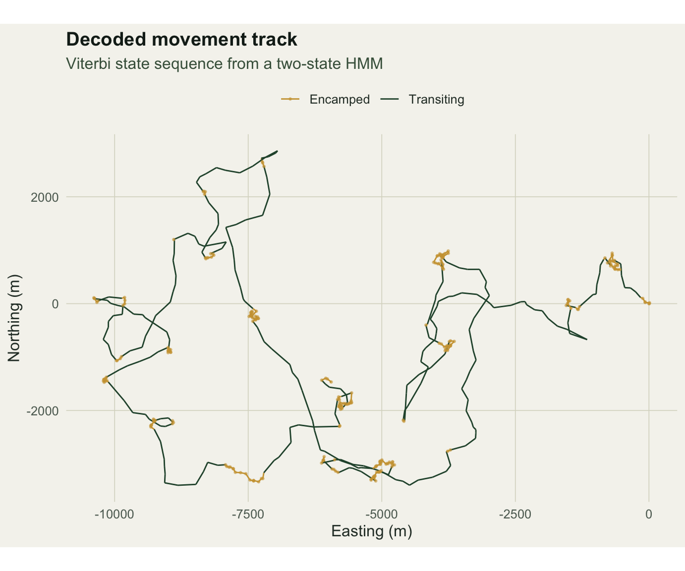
Against the known truth the decoded path is right 0.956 of the time.
What the naive threshold misses
The naive classifier uses step length alone. We put the threshold where the two fitted state densities cross, weighted by how often each state occurs, which is the best a step-only rule can do. Then we compare.
grid <- seq(min(step), max(step), length.out = 20000)
d1 <- delta_hat[1] * dgamma(grid, shape = p_hat$shape[1], scale = p_hat$scale[1])
d2 <- delta_hat[2] * dgamma(grid, shape = p_hat$shape[2], scale = p_hat$scale[2])
cross <- grid[which(diff(sign(d2 - d1)) != 0)]
thr <- cross[cross > p_hat$shape[1] * p_hat$scale[1]][1]
naive <- ifelse(step > thr, 2, 1)
switches <- function(z) sum(diff(z) != 0)
The threshold sits at 94 m. The naive rule is right 0.914 of the time, below Viterbi’s 0.956. The gap is larger than it looks, because the two rules fail differently. The true path switches state 66 times; Viterbi switches 62 times, close to the truth; the naive rule switches 126 times, roughly double. With no memory, every long step in a foraging bout and every short step in a transit is read as an instantaneous change of behaviour, so the naive path flickers. There are 30 steps the threshold gets wrong that Viterbi gets right, against only 9 the other way. The HMM wins because it uses the turning angle as a second signal and because the Markov chain penalises isolated flips.
The state-dependent distributions
The fitted emissions are what separate the states. The gamma densities for step length barely overlap at their modes, and the von Mises densities for turning angle are a sharp forward peak against a near-flat spread.
sx <- seq(0, max(step), length.out = 300); tx <- seq(-pi, pi, length.out = 300)
obs <- rbind(data.frame(val = step, panel = "Step length (m)"),
             data.frame(val = turn[!is.na(turn)], panel = "Turning angle (rad)"))
cur <- rbind(
  data.frame(val = sx, dens = delta_hat[1] * dgamma(sx, p_hat$shape[1], scale = p_hat$scale[1]), state = "Encamped",  panel = "Step length (m)"),
  data.frame(val = sx, dens = delta_hat[2] * dgamma(sx, p_hat$shape[2], scale = p_hat$scale[2]), state = "Transiting", panel = "Step length (m)"),
  data.frame(val = tx, dens = delta_hat[1] * dvm(tx, 0, p_hat$kappa[1]), state = "Encamped",  panel = "Turning angle (rad)"),
  data.frame(val = tx, dens = delta_hat[2] * dvm(tx, 0, p_hat$kappa[2]), state = "Transiting", panel = "Turning angle (rad)"))
ggplot() +
  geom_histogram(data = obs, aes(val, after_stat(density)), bins = 40, fill = pal$sage, alpha = 0.32) +
  geom_line(data = cur, aes(val, dens, colour = state), linewidth = 0.9) +
  facet_wrap(~panel, scales = "free") +
  scale_colour_manual(values = state_cols, name = NULL) +
  labs(title = "State-dependent emission distributions",
       subtitle = "Fitted gamma (step length) and von Mises (turning angle) per state",
       x = NULL, y = "Density") + theme_te()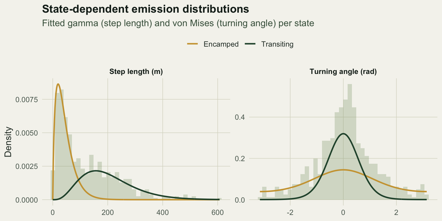
When this helps, and when to be careful
Two states are a modelling choice, not a fact about the animal, and this is where care is needed. The number of states is not known in advance, and adding more will always raise the likelihood; choosing it well is a separate problem, covered in the companion post on state selection. The emissions matter too: gamma and von Mises are conventional for step lengths and turning angles, but a bimodal or zero-inflated step distribution needs more thought. Coarse or irregular fixes change step lengths and turning angles in ways that blur the states, so the sampling interval is part of the model. Finally, a fitted state is a statistical cluster in step-and-turn space; calling it “foraging” is a biological interpretation that the model cannot supply on its own.
Even so, the pattern is worth the effort. A latent-state model reads the sequence as a sequence, and it uses every stream of information at once, which a threshold on a single variable cannot do.
References
Baum, L. E., Petrie, T., Soules, G., & Weiss, N. (1970). A maximization technique occurring in the statistical analysis of probabilistic functions of Markov chains. The Annals of Mathematical Statistics, 41(1), 164-171. https://doi.org/10.1214/aoms/1177697196
Langrock, R., King, R., Matthiopoulos, J., Thomas, L., Fortin, D., & Morales, J. M. (2012). Flexible and practical modeling of animal telemetry data: hidden Markov models and extensions. Ecology, 93(11), 2336-2342. https://doi.org/10.1890/11-2241.1
McClintock, B. T., Langrock, R., Gimenez, O., Cam, E., Borchers, D. L., Glennie, R., & Patterson, T. A. (2020). Uncovering ecological state dynamics with hidden Markov models. Ecology Letters, 23(12), 1878-1903. https://doi.org/10.1111/ele.13610
Michelot, T., Langrock, R., & Patterson, T. A. (2016). moveHMM: an R package for the statistical modelling of animal movement data using hidden Markov models. Methods in Ecology and Evolution, 7(11), 1308-1315. https://doi.org/10.1111/2041-210X.12578
Morales, J. M., Haydon, D. T., Frair, J., Holsinger, K. E., & Fryxell, J. M. (2004). Extracting more out of relocation data: building movement models as mixtures of random walks. Ecology, 85(9), 2436-2445. https://doi.org/10.1890/03-0269
Patterson, T. A., Thomas, L., Wilcox, C., Ovaskainen, O., & Matthiopoulos, J. (2008). State-space models of individual animal movement. Trends in Ecology & Evolution, 23(2), 87-94. https://doi.org/10.1016/j.tree.2007.10.009
Viterbi, A. (1967). Error bounds for convolutional codes and an asymptotically optimum decoding algorithm. IEEE Transactions on Information Theory, 13(2), 260-269. https://doi.org/10.1109/TIT.1967.1054010
Zucchini, W., MacDonald, I. L., & Langrock, R. (2016). Hidden Markov Models for Time Series: An Introduction Using R (2nd ed.). CRC Press. ISBN 978-1-4822-5383-2.