library(ggplot2)
library(dplyr)

pal <- list(ink = "#16241d", body = "#2c3a31", forest = "#275139", label = "#46604a",
            sage = "#93a87f", paper = "#f5f4ee", line = "#dad9ca", faint = "#5d6b61")
theme_te <- function(base_size = 12) {
  theme_minimal(base_size = base_size) +
    theme(plot.background = element_rect(fill = pal$paper, colour = NA),
          panel.background = element_rect(fill = pal$paper, colour = NA),
          panel.grid.major = element_line(colour = pal$line, linewidth = 0.3),
          panel.grid.minor = element_blank(),
          axis.text = element_text(colour = pal$faint), axis.title = element_text(colour = pal$body),
          plot.title = element_text(colour = pal$ink, face = "bold"),
          plot.subtitle = element_text(colour = pal$label),
          strip.text = element_text(colour = pal$ink, face = "bold"),
          legend.text = element_text(colour = pal$body), legend.position = "top")
}
dvm <- function(theta, mu, kappa) exp(kappa * cos(theta - mu)) / (2 * pi * besselI(kappa, 0))
rvm <- function(n, mu, kappa) {
  mu <- rep(mu, length.out = n); kappa <- rep(kappa, length.out = n); out <- numeric(n)
  for (i in 1:n) {
    k <- kappa[i]; a <- 1 + sqrt(1 + 4 * k^2); b <- (a - sqrt(2 * a)) / (2 * k); r <- (1 + b^2) / (2 * b)
    repeat {
      u1 <- runif(1); u2 <- runif(1); u3 <- runif(1)
      z <- cos(pi * u1); f <- (1 + r * z) / (r + z); cc <- k * (r - f)
      if (cc * (2 - cc) - u2 > 0 || log(cc / u2) + 1 - cc >= 0) { out[i] <- sign(u3 - 0.5) * acos(f) + mu[i]; break }
    }
  }
  ((out + pi) %% (2 * pi)) - pi
}

Gamma_true <- matrix(c(0.90, 0.10, 0.15, 0.85), 2, 2, byrow = TRUE)
shape_true <- c(2, 4); scale_true <- c(20, 50); kappa_true <- c(0.7, 3.0); Tn <- 500
delta_true <- solve(t(diag(2) - Gamma_true + 1), rep(1, 2))
set.seed(4517)
S <- integer(Tn); S[1] <- sample(1:2, 1, prob = delta_true)
for (t in 2:Tn) S[t] <- sample(1:2, 1, prob = Gamma_true[S[t - 1], ])
step <- rgamma(Tn, shape = shape_true[S], scale = scale_true[S])
phi  <- rvm(Tn, 0, kappa_true[S]); turn <- phi; turn[1] <- NA

w2n <- function(w) { g12 <- plogis(w[1]); g21 <- plogis(w[2])
  list(Gamma = matrix(c(1 - g12, g12, g21, 1 - g21), 2, 2, byrow = TRUE),
       shape = exp(w[c(3, 5)]), scale = exp(w[c(4, 6)]), kappa = exp(w[c(7, 8)])) }
allprobs <- function(p) { ap <- matrix(1, Tn, 2)
  for (j in 1:2) ap[, j] <- dgamma(step, shape = p$shape[j], scale = p$scale[j]) *
    ifelse(is.na(turn), 1, dvm(turn, 0, p$kappa[j]))
  ap }
nll <- function(w) { p <- w2n(w); ap <- allprobs(p)
  delta <- solve(t(diag(2) - p$Gamma + 1), rep(1, 2))
  foo <- delta * ap[1, ]; s <- sum(foo); ls <- log(s); foo <- foo / s
  for (t in 2:Tn) { foo <- (foo %*% p$Gamma) * ap[t, ]; s <- sum(foo); ls <- ls + log(s); foo <- foo / s }
  -ls }
w0 <- c(qlogis(0.1), qlogis(0.15), log(2), log(25), log(4), log(45), log(0.8), log(2.5))
fit <- optim(w0, nll, method = "Nelder-Mead", control = list(maxit = 5000, reltol = 1e-12))
fit <- optim(fit$par, nll, method = "BFGS", control = list(maxit = 1000, reltol = 1e-12))
p2 <- w2n(fit$par)Checking a movement HMM
ecology tutorial
movement ecology
hidden markov models
Two checks every fitted movement HMM needs: forecast pseudo-residuals to test the model, and forward-backward posterior probabilities to see the uncertainty Viterbi hides.
A fitted HMM returns parameters and a decoded state sequence, and both invite too much trust. The parameters come from whichever model you chose, which may be the wrong one; the decoded path is a single best guess presented without any sense of how firm it is. Two checks address these directly. Forecast pseudo-residuals ask whether the fitted model actually describes the data. The forward-backward algorithm replaces the single Viterbi path with a probability for each state at each step, so the model can tell you where it is sure and where it is guessing. This post applies both to the two-state track from the foundation post.
Setup and the fitted model
We re-simulate and re-fit the two-state model so the post stands alone.
Forward-backward: probabilities, not a path
Viterbi gives the single most probable path. The forward-backward algorithm gives something more useful for checking: the smoothed probability \(\Pr(S_t = j \mid \text{all data})\) at every step. It runs the scaled forward recursion, a matching backward recursion, and multiplies the two. It also gives the one-step-ahead predictive distribution we will need for residuals, and its scaling constants reproduce the log-likelihood as a side check.
fwd_bwd <- function(p) {
  ap <- allprobs(p); delta <- solve(t(diag(2) - p$Gamma + 1), rep(1, 2))
  phi <- matrix(NA, Tn, 2); cvec <- numeric(Tn)
  foo <- delta * ap[1, ]; cvec[1] <- sum(foo); phi[1, ] <- foo / cvec[1]
  for (t in 2:Tn) { foo <- (phi[t - 1, ] %*% p$Gamma) * ap[t, ]; cvec[t] <- sum(foo); phi[t, ] <- foo / cvec[t] }
  bt <- matrix(NA, Tn, 2); bt[Tn, ] <- 1
  for (t in (Tn - 1):1) bt[t, ] <- as.numeric(p$Gamma %*% (ap[t + 1, ] * bt[t + 1, ])) / cvec[t + 1]
  post <- phi * bt; post <- post / rowSums(post)
  xi <- matrix(NA, Tn, 2); xi[1, ] <- delta
  for (t in 2:Tn) xi[t, ] <- as.numeric(phi[t - 1, ] %*% p$Gamma)
  list(post = post, xi = xi, llk = sum(log(cvec)))
}
fb <- fwd_bwd(p2)
For the single best path we also run Viterbi, exactly as in the foundation post.
viterbi <- function(p) {
  ap <- allprobs(p); delta <- solve(t(diag(2) - p$Gamma + 1), rep(1, 2))
  xi <- matrix(0, Tn, 2); foo <- delta * ap[1, ]; xi[1, ] <- foo / sum(foo)
  for (t in 2:Tn) { foo <- apply(xi[t - 1, ] * p$Gamma, 2, max) * ap[t, ]; xi[t, ] <- foo / sum(foo) }
  iv <- integer(Tn); iv[Tn] <- which.max(xi[Tn, ])
  for (t in (Tn - 1):1) iv[t] <- which.max(p$Gamma[, iv[t + 1]] * xi[t, ]); iv
}
vit <- viterbi(p2)
loc <- apply(fb$post, 1, which.max)
The log-likelihood recovered from the scaling constants is 3478.33, matching the fitted value to the decimal. The smoothed probabilities let us decode a second way, by taking the most probable state at each step (local decoding) rather than the most probable whole path. Here the two agree 0.996 of the time, but where they disagree is exactly where the model is unsure.
The uncertainty Viterbi hides
Plotting the posterior probability of the transiting state across a stretch of the track shows the point. Most of the time it sits hard against zero or one and the Viterbi path runs along it. At the behavioural transitions it lifts off, and there the single path is a coin toss dressed up as a decision.
maxpost <- apply(fb$post, 1, max)
w <- 1:170
dfd <- data.frame(t = w, post = fb$post[w, 2], vit = as.numeric(vit[w] == 2),
                  truth = factor(ifelse(S[w] == 2, "Transiting", "Encamped"), levels = c("Encamped", "Transiting")))
unc <- dfd[dfd$post > 0.2 & dfd$post < 0.8, ]
ggplot(dfd, aes(t)) +
  geom_tile(aes(y = -0.06, fill = truth), height = 0.06) +
  geom_rect(data = unc, aes(xmin = t - 0.5, xmax = t + 0.5, ymin = 0, ymax = 1), fill = "#cda23f", alpha = 0.18, inherit.aes = FALSE) +
  geom_step(aes(y = vit), colour = pal$faint, linewidth = 0.5, direction = "mid") +
  geom_line(aes(y = post), colour = "#275139", linewidth = 0.9) +
  scale_fill_manual(values = c(Encamped = "#cda23f", Transiting = "#275139"), name = "True state") +
  scale_y_continuous(breaks = c(0, 0.5, 1)) +
  labs(title = "Decoding uncertainty the Viterbi path hides",
       subtitle = "Green: posterior P(transiting); grey step: single Viterbi path; band: true state; shaded: ambiguous steps",
       x = "Step index", y = "P(transiting)") + theme_te()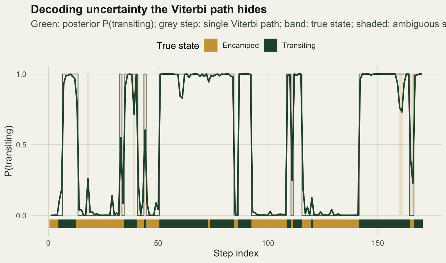
Across the whole track the mean of the top state probability is 0.97, so decoding is usually confident. But 6% of steps have their best state below 0.8 probability, and those steps cluster at the transitions. Reporting a single path throws that information away; carrying the posterior keeps it, which matters whenever the decoded states feed a downstream analysis.
Forecast pseudo-residuals
A residual for an HMM cannot be an observed minus a fitted value, because the observations are not normal and the state is latent. The device that works is the probability integral transform. For each step we form the one-step-ahead forecast distribution, a mixture over states weighted by the predictive probabilities from the filter, evaluate its cumulative distribution at the observed value, and map the result through the normal quantile function. If the model is right these pseudo-residuals are standard normal and independent, so a normal quantile plot and the residual autocorrelation are the two things to look at.
Fstep2 <- fb$xi[, 1] * pgamma(step, shape = p2$shape[1], scale = p2$scale[1]) +
          fb$xi[, 2] * pgamma(step, shape = p2$shape[2], scale = p2$scale[2])
r_step2 <- qnorm(pmin(pmax(Fstep2, 1e-10), 1 - 1e-10))
qqcor <- function(r) cor(sort(r), qnorm(ppoints(length(r))))
acf1  <- function(r) acf(r, plot = FALSE, lag.max = 1)$acf[2]
For the step lengths the two-state model looks right: the pseudo-residuals have a normal quantile correlation of 0.999, 4% fall outside the central 95% band, close to the 5% expected, and their lag-one autocorrelation is -0.034, effectively zero. The Markov structure has absorbed the persistence, leaving white residuals.
What a wrong model looks like
The check earns its place by failing when the model is wrong. We fit a one-state model, a single gamma and von Mises with no switching, and run the same residuals. A single gamma cannot be both short and long at once, and with no states it cannot represent the runs of similar steps, so the residuals should show it.
nll1 <- function(w) { sh <- exp(w[1]); sc <- exp(w[2]); ka <- exp(w[3])
  d <- dgamma(step, shape = sh, scale = sc) * ifelse(is.na(turn), 1, dvm(turn, 0, ka))
  -sum(log(pmax(d, 1e-300))) }
f1 <- optim(c(log(mean(step)^2 / var(step)), log(var(step) / mean(step)), log(1)), nll1,
            method = "Nelder-Mead", control = list(maxit = 2000, reltol = 1e-11))
p1 <- list(shape = exp(f1$par[1]), scale = exp(f1$par[2]), kappa = exp(f1$par[3]))
r_step1 <- qnorm(pmin(pmax(pgamma(step, shape = p1$shape, scale = p1$scale), 1e-10), 1 - 1e-10))
The one-state fit is far worse on likelihood, with a negative log-likelihood of 3642 against 3478.3 for two states. Its step residuals are only slightly less normal by the quantile correlation, 0.994, which on its own might not raise an alarm. The autocorrelation is where it breaks: the lag-one value is 0.48, an order of magnitude larger than the two-state model’s and a clear sign that structure remains in the residuals. This is the pattern to watch for. A model that misses the state dynamics leaves the dependence in the residuals even when the marginal shape looks passable.
qqdat <- function(r, lab) data.frame(theo = qnorm(ppoints(length(r))), samp = sort(r), model = lab)
qq <- rbind(qqdat(r_step2, "Two-state model"), qqdat(r_step1, "One-state model"))
qq$model <- factor(qq$model, levels = c("Two-state model", "One-state model"))
ann <- data.frame(model = factor(c("Two-state model", "One-state model"), levels = levels(qq$model)),
                  lab = c(paste0("lag-1 ACF = ", round(acf1(r_step2), 2)),
                          paste0("lag-1 ACF = ", round(acf1(r_step1), 2))))
ggplot(qq, aes(theo, samp)) +
  geom_abline(slope = 1, intercept = 0, colour = pal$faint, linetype = "dashed") +
  geom_point(colour = "#275139", size = 0.8, alpha = 0.6) +
  geom_text(data = ann, aes(x = -2.7, y = 3.1, label = lab), hjust = 0, size = 3.4, colour = pal$ink) +
  facet_wrap(~model) +
  labs(title = "Pseudo-residual check of the step distribution",
       subtitle = "The one-state model leaves strong residual autocorrelation the two-state model removes",
       x = "Theoretical normal quantile", y = "Pseudo-residual") + theme_te()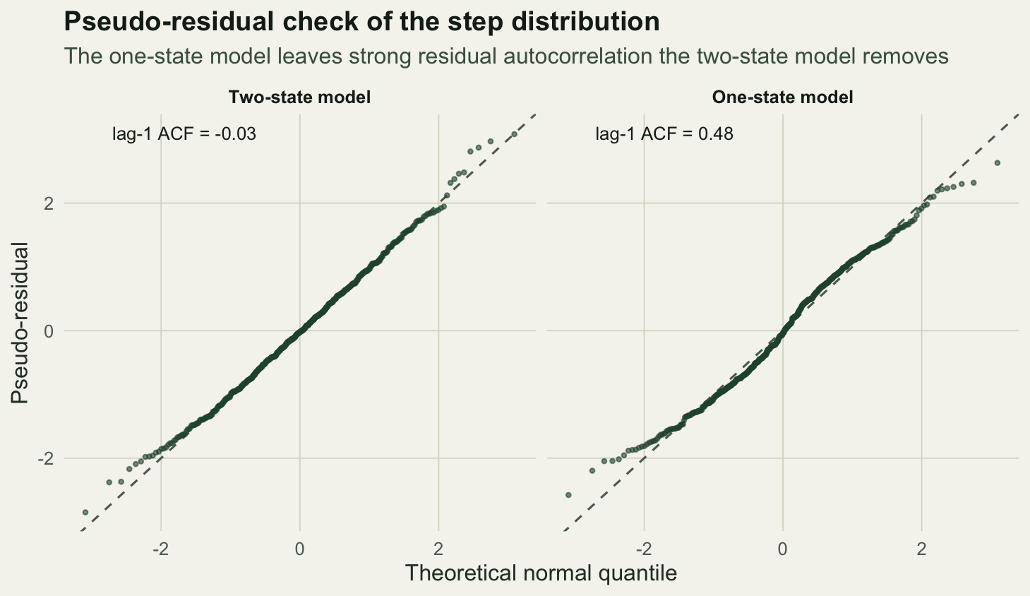
The turning angles, and a closing note
The same residuals apply to the turning angles, using a numerical von Mises cumulative distribution in place of the gamma one.
gg <- seq(-pi, pi, length.out = 4000)
vmcdf_fun <- function(kappa) {
  dens <- dvm(gg, 0, kappa)
  cdf <- c(0, cumsum((dens[-1] + dens[-length(dens)]) / 2 * diff(gg))); cdf <- cdf / cdf[length(cdf)]
  approxfun(gg, cdf, rule = 2)
}
c1 <- vmcdf_fun(p2$kappa[1]); c2 <- vmcdf_fun(p2$kappa[2]); ok <- !is.na(turn)
Fturn <- fb$xi[ok, 1] * c1(turn[ok]) + fb$xi[ok, 2] * c2(turn[ok])
r_turn2 <- qnorm(pmin(pmax(Fturn, 1e-10), 1 - 1e-10))
For the two-state model the turn residuals are also close to normal, with a quantile correlation of 0.998, so both emission streams check out.
Neither check is a certificate. Pseudo-residuals can look fine for a model that is still wrong in a way the data cannot reveal, and a confident posterior can be confidently wrong if the emissions are misspecified. But the two together catch the common failures: residual autocorrelation flags missing state structure, tail departures flag the wrong emission family, and the posterior shows where any decoded sequence should be read with caution. Fit the model, then check it; the decoded track is a conclusion, not a given.
References
Zucchini, W., MacDonald, I. L., & Langrock, R. (2016). Hidden Markov Models for Time Series: An Introduction Using R (2nd ed.). CRC Press. ISBN 978-1-4822-5383-2.
Langrock, R., King, R., Matthiopoulos, J., Thomas, L., Fortin, D., & Morales, J. M. (2012). Flexible and practical modeling of animal telemetry data: hidden Markov models and extensions. Ecology, 93(11), 2336-2342. https://doi.org/10.1890/11-2241.1
McClintock, B. T., Langrock, R., Gimenez, O., Cam, E., Borchers, D. L., Glennie, R., & Patterson, T. A. (2020). Uncovering ecological state dynamics with hidden Markov models. Ecology Letters, 23(12), 1878-1903. https://doi.org/10.1111/ele.13610
Michelot, T., Langrock, R., & Patterson, T. A. (2016). moveHMM: an R package for the statistical modelling of animal movement data using hidden Markov models. Methods in Ecology and Evolution, 7(11), 1308-1315. https://doi.org/10.1111/2041-210X.12578