library(ggplot2)
library(dplyr)
library(tidyr)

pal <- list(ink = "#16241d", body = "#2c3a31", forest = "#275139", label = "#46604a",
            sage = "#93a87f", paper = "#f5f4ee", line = "#dad9ca", faint = "#5d6b61")
theme_te <- function(base_size = 12) {
  theme_minimal(base_size = base_size) +
    theme(plot.background = element_rect(fill = pal$paper, colour = NA),
          panel.background = element_rect(fill = pal$paper, colour = NA),
          panel.grid.major = element_line(colour = pal$line, linewidth = 0.3),
          panel.grid.minor = element_blank(),
          axis.text = element_text(colour = pal$faint), axis.title = element_text(colour = pal$body),
          plot.title = element_text(colour = pal$ink, face = "bold"),
          plot.subtitle = element_text(colour = pal$label),
          legend.text = element_text(colour = pal$body), legend.position = "top")
}
dvm <- function(theta, mu, kappa) exp(kappa * cos(theta - mu)) / (2 * pi * besselI(kappa, 0))
rvm <- function(n, mu, kappa) {
  mu <- rep(mu, length.out = n); kappa <- rep(kappa, length.out = n); out <- numeric(n)
  for (i in 1:n) {
    k <- kappa[i]; a <- 1 + sqrt(1 + 4 * k^2); b <- (a - sqrt(2 * a)) / (2 * k); r <- (1 + b^2) / (2 * b)
    repeat {
      u1 <- runif(1); u2 <- runif(1); u3 <- runif(1)
      z <- cos(pi * u1); f <- (1 + r * z) / (r + z); cc <- k * (r - f)
      if (cc * (2 - cc) - u2 > 0 || log(cc / u2) + 1 - cc >= 0) { out[i] <- sign(u3 - 0.5) * acos(f) + mu[i]; break }
    }
  }
  ((out + pi) %% (2 * pi)) - pi
}
# time-varying two-state transition matrix from the covariate
mkG <- function(b, x) { g12 <- plogis(b[1] + b[2] * x); g21 <- plogis(b[3] + b[4] * x)
matrix(c(1 - g12, g12, g21, 1 - g21), 2, 2, byrow = TRUE) }Covariates in a movement HMM
ecology tutorial
movement ecology
hidden markov models
Let HMM transition probabilities depend on time of day through a multinomial logit, recover a diurnal activity budget, and see what a homogeneous model hides.
An animal does not switch between behaviours at a constant rate. It is more likely to start travelling at some times of day than others, more likely to settle at others. A movement HMM with a fixed transition matrix cannot express this: it reports one average switching rate and calls the job done. Letting the transition probabilities depend on a covariate turns the same model into a description of when behaviour changes, not just how often. This post puts time of day on the transitions of a two-state movement HMM through a multinomial logit, recovers a diurnal activity budget, and shows what the homogeneous model leaves on the table.
Covariate-dependent transitions
With two states there are two switching probabilities to model: \(\gamma_{12}\), the chance of leaving the encamped state for the transiting one, and \(\gamma_{21}\), the chance of settling back. Each is tied to the covariate \(x_t\) through a logit,
\[\gamma_{12}(x_t) = \operatorname{logit}^{-1}(\beta_0^{12} + \beta_1^{12}\,x_t), \qquad \gamma_{21}(x_t) = \operatorname{logit}^{-1}(\beta_0^{21} + \beta_1^{21}\,x_t),\]
so the transition matrix changes at every step. The covariate is a diurnal term, \(x_t = \cos(2\pi\,h_t / 24)\) for hour of day \(h_t\), which peaks at midday and troughs at midnight. The emission distributions are unchanged from the foundation post; only the transitions carry the covariate.
Setup
A track with a diurnal rhythm
We simulate 1200 steps at half-hour intervals. The true coefficients make the animal likely to start travelling by day and to settle by night, so activity should rise and fall on a daily cycle.
b_true <- c(-2.20, 1.60, -1.75, -1.30)              # b0_12, b1_12, b0_21, b1_21
shape_true <- c(2, 4); scale_true <- c(20, 50); kappa_true <- c(0.7, 3.0)
Tn <- 1200
hour <- ((0:(Tn - 1)) * 0.5) %% 24
cov  <- cos(2 * pi * hour / 24)

set.seed(7731)
S <- integer(Tn)
G1 <- mkG(b_true, cov[1]); d1 <- solve(t(diag(2) - G1 + 1), rep(1, 2)); S[1] <- sample(1:2, 1, prob = d1)
for (t in 2:Tn) S[t] <- sample(1:2, 1, prob = mkG(b_true, cov[t])[S[t - 1], ])
step <- rgamma(Tn, shape = shape_true[S], scale = scale_true[S])
phi  <- rvm(Tn, 0, kappa_true[S]); turn <- phi; turn[1] <- NA
The rhythm is already visible in the raw states: the animal is transiting 0.72 of the time when the covariate is positive (the daylight half of the cycle) against 0.2 when it is negative.
Two likelihoods: covariate and homogeneous
The covariate likelihood is the forward algorithm with a fresh transition matrix at each step. The homogeneous baseline is the same code with the covariate slopes forced to zero, so it estimates a single constant transition matrix. Fitting both lets us test whether the diurnal term earns its two extra parameters.
nll_cov <- function(w, step, turn, cov) {
  b <- w[1:4]; sh <- exp(w[5:6]); sc <- exp(w[7:8]); ka <- exp(w[9:10]); Tn <- length(step)
  ap <- matrix(1, Tn, 2)
  for (j in 1:2) ap[, j] <- dgamma(step, sh[j], scale = sc[j]) * ifelse(is.na(turn), 1, dvm(turn, 0, ka[j]))
  if (any(!is.finite(ap))) return(1e10)
  G1 <- mkG(b, cov[1]); delta <- solve(t(diag(2) - G1 + 1), rep(1, 2))
  foo <- delta * ap[1, ]; s <- sum(foo); if (s <= 0) return(1e10); ls <- log(s); foo <- foo / s
  for (t in 2:Tn) { Gt <- mkG(b, cov[t]); foo <- (foo %*% Gt) * ap[t, ]; s <- sum(foo); if (s <= 0) return(1e10); ls <- ls + log(s); foo <- foo / s }
  -ls
}
nll_hom <- function(w, step, turn) nll_cov(c(w[1], 0, w[2], 0, w[3:8]), step, turn, rep(0, length(step)))
w0c <- c(-2, 1, -1.5, -1, log(2), log(4), log(20), log(50), log(0.7), log(3))
fc <- optim(w0c, nll_cov, step = step, turn = turn, cov = cov, method = "Nelder-Mead",
control = list(maxit = 4000, reltol = 1e-11))
fc <- optim(fc$par, nll_cov, step = step, turn = turn, cov = cov, method = "BFGS",
control = list(maxit = 300, reltol = 1e-12))
w0h <- c(-2, -1.5, log(2), log(4), log(20), log(50), log(0.7), log(3))
fh <- optim(w0h, nll_hom, step = step, turn = turn, method = "Nelder-Mead",
control = list(maxit = 4000, reltol = 1e-11))
fh <- optim(fh$par, nll_hom, step = step, turn = turn, method = "BFGS",
control = list(maxit = 300, reltol = 1e-12))
bh <- fc$par[1:4]The covariate model recovers the truth well: the fitted coefficients are -2.18, 1.46, -1.81 and -1.14 against a truth of -2.2, 1.6, -1.75 and -1.3. The positive slope on \(\gamma_{12}\) and the negative slope on \(\gamma_{21}\) together say what the biology said: travel starts by day, settling happens at night. The homogeneous model, by contrast, can only report averages, a constant 0.084 chance of starting to travel and a constant 0.102 chance of settling, with the daily pattern folded away.
kC <- 10; kH <- 8
aic_c <- 2 * fc$value + 2 * kC; aic_h <- 2 * fh$value + 2 * kH
lr <- 2 * (fh$value - fc$value)
The covariate model wins decisively. Its AIC is 16346.4 against 16412.7 for the homogeneous model, a gap of 66.3. A likelihood ratio test of the two nested models gives a statistic of 70.3 on 2 degrees of freedom, with a p-value of 5.3^{-16}. The diurnal signal is real and the homogeneous model was hiding it.
The recovered response curves
The point of the covariate model is that it gives a curve, not a constant. We plot each transition probability across the day, with the homogeneous constants as dotted lines to show what was lost.
hr <- seq(0, 24, length.out = 200); cx <- cos(2 * pi * hr / 24)
mkg <- function(b, x, which) if (which == 12) plogis(b[1] + b[2] * x) else plogis(b[3] + b[4] * x)
g12h <- plogis(fh$par[1]); g21h <- plogis(fh$par[2])
dfp <- rbind(
  data.frame(hour = hr, prob = mkg(bh, cx, 12), tr = "Start transiting", src = "Covariate model"),
  data.frame(hour = hr, prob = mkg(bh, cx, 21), tr = "Settle",          src = "Covariate model"),
  data.frame(hour = hr, prob = mkg(b_true, cx, 12), tr = "Start transiting", src = "Truth"),
  data.frame(hour = hr, prob = mkg(b_true, cx, 21), tr = "Settle",          src = "Truth"))
hom <- data.frame(tr = c("Start transiting", "Settle"), y = c(g12h, g21h))
ggplot(dfp, aes(hour, prob, colour = tr, linetype = src)) +
  geom_hline(data = hom, aes(yintercept = y, colour = tr), linetype = "dotted", linewidth = 0.6) +
  geom_line(linewidth = 0.9) +
  scale_colour_manual(values = c("Start transiting" = "#b5534e", "Settle" = "#275139"), name = NULL) +
  scale_linetype_manual(values = c("Covariate model" = "solid", "Truth" = "22"), name = NULL) +
  scale_x_continuous(breaks = seq(0, 24, 6)) +
  labs(title = "Transition probabilities vary with time of day",
       subtitle = "Dotted lines: the single constant each transition takes in a homogeneous model",
       x = "Hour of day", y = "Transition probability") + theme_te()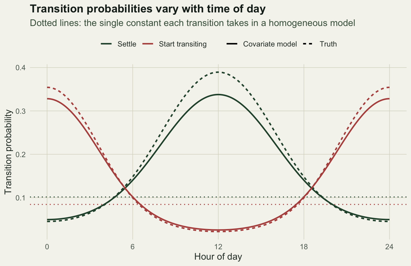
From transitions to a budget
Transition probabilities are the mechanics; the quantity a reader wants is the share of time spent in each behaviour, and how it moves through the day. At any fixed covariate value the transition matrix has its own stationary distribution, so we can read the activity budget straight off the fitted coefficients: the stationary probability of the transiting state is \(\gamma_{12}(x) / (\gamma_{12}(x) + \gamma_{21}(x))\). Plotting it against the hour, beside the binned empirical proportions, shows the model tracing the daily cycle that the homogeneous flat line cannot.
statP2 <- function(b, x) { g12 <- plogis(b[1] + b[2] * x); g21 <- plogis(b[3] + b[4] * x); g12 / (g12 + g21) }
budget <- data.frame(hour = hr, model = statP2(bh, cx), truth = statP2(b_true, cx))
homP <- g12h / (g12h + g21h)
brks <- cut(hour, breaks = seq(0, 24, 2), include.lowest = TRUE)
emp <- data.frame(hour = tapply(hour, brks, mean), p = tapply(S == 2, brks, mean))
ggplot(budget, aes(hour)) +
  geom_hline(yintercept = homP, linetype = "dotted", colour = pal$faint, linewidth = 0.7) +
  annotate("text", x = 1.2, y = homP + 0.03, label = "homogeneous", hjust = 0, size = 3.2, colour = pal$faint) +
  geom_line(aes(y = truth), linetype = "22", colour = pal$sage, linewidth = 0.9) +
  geom_line(aes(y = model), colour = "#275139", linewidth = 1.1) +
  geom_point(data = emp, aes(hour, p), colour = "#b5534e", size = 2.2) +
  scale_x_continuous(breaks = seq(0, 24, 6)) + ylim(0, 1) +
  labs(title = "Diurnal activity budget",
       subtitle = "Stationary probability of transiting: model (green), truth (pale dashed), binned data (points)",
       x = "Hour of day", y = "P(transiting)") + theme_te()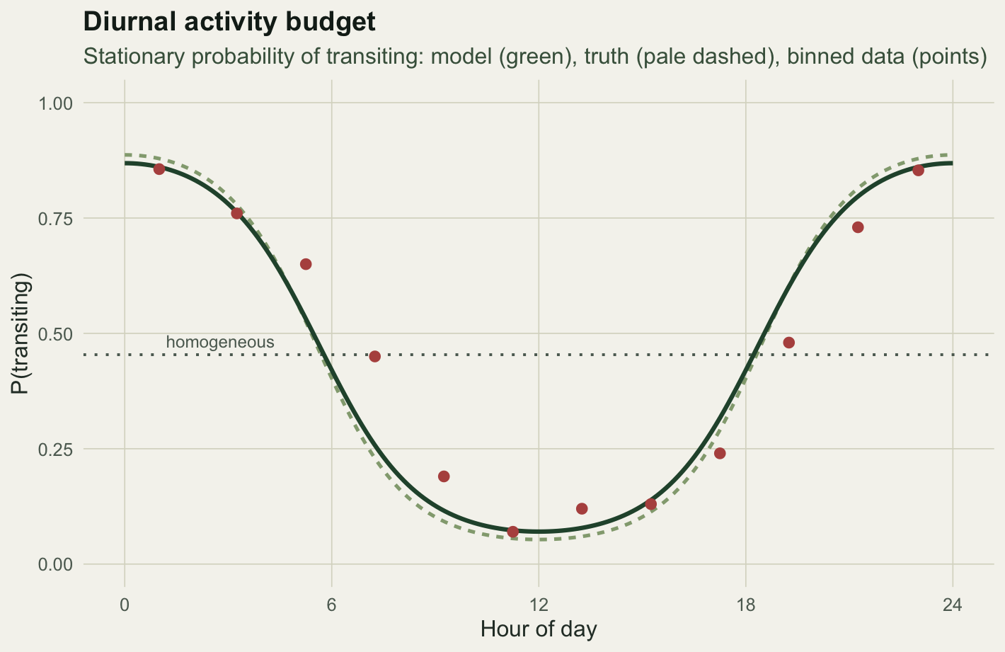
Notes and cautions
The covariate here goes on the transitions, which is the usual and the interpretable choice: it changes when behaviour switches. A covariate can instead be put on the emissions, changing what a behaviour looks like, but the two are different claims and should not be swapped casually. A cyclic covariate needs a cyclic construction; the single cosine term used here is the simplest, and a richer daily shape would need more harmonics or a spline. As always, correlation with time of day is not proof of a causal driver, and a covariate that merely tracks an unmodelled variable will still improve the fit. The stationary budget, finally, is the long-run share implied by the transition matrix at a fixed covariate value, which is a clean summary but not the same as the realised occupancy over a finite track.
References
Langrock, R., King, R., Matthiopoulos, J., Thomas, L., Fortin, D., & Morales, J. M. (2012). Flexible and practical modeling of animal telemetry data: hidden Markov models and extensions. Ecology, 93(11), 2336-2342. https://doi.org/10.1890/11-2241.1
Patterson, T. A., Basson, M., Bravington, M. V., & Gunn, J. S. (2009). Classifying movement behaviour in relation to environmental conditions using hidden Markov models. Journal of Animal Ecology, 78(6), 1113-1123. https://doi.org/10.1111/j.1365-2656.2009.01583.x
Michelot, T., Langrock, R., & Patterson, T. A. (2016). moveHMM: an R package for the statistical modelling of animal movement data using hidden Markov models. Methods in Ecology and Evolution, 7(11), 1308-1315. https://doi.org/10.1111/2041-210X.12578
Zucchini, W., MacDonald, I. L., & Langrock, R. (2016). Hidden Markov Models for Time Series: An Introduction Using R (2nd ed.). CRC Press. ISBN 978-1-4822-5383-2.