The storage effect and coexistence

The storage effect in R: how a fluctuating environment lets competitors coexist through the lottery model, buffered growth, and a rare-species advantage.

A constant environment is unkind to coexistence. Classical competition theory says that when two species compete for the same thing, the better competitor wins and the other is squeezed out; the only escape is for the species to differ, to want different resources or suffer different enemies. So it is a surprise that a varying environment, one that shifts the advantage from one species to another and back, can hold competitors together that a constant environment would separate. That mechanism is the storage effect, and it is one of the central ideas in how fluctuations maintain diversity.

A lottery for space

The cleanest model is the lottery (Chesson and Warner 1981 The American Naturalist 117(6):923-943). Picture a saturated community where every site is occupied by an adult. Adults die at rate 0.1 per year, opening sites, and the open sites are won by recruits in proportion to how many each species produces that year. The environment sets the reproductive output: a good year for one species is a bad year for the other. Track the fraction of sites held by species 1.

delta <- 0.1
states <- list(c(3, 0.5), c(0.5, 3))            # (output sp1, output sp2) in each environmental state
step <- function(p, s, d) {
  share <- (s[1]*p) / (s[1]*p + s[2]*(1-p))      # fraction of open sites won by sp1 recruits
  (1 - d)*p + d*share                            # surviving adults plus recruits into open sites
}
# rare species 1 (starts at 0.10) in a constant average environment vs a fluctuating one
set.seed(11)
p_const <- 0.10; for (t in 1:300) p_const <- step(p_const, c(1.75, 1.75), delta)
p_fluc  <- 0.10; for (t in 1:300) p_fluc  <- step(p_fluc, states[[sample(2, 1)]], delta)
c(constant = round(p_const, 3), fluctuating = round(p_fluc, 3))

   constant fluctuating 
      0.100       0.576 

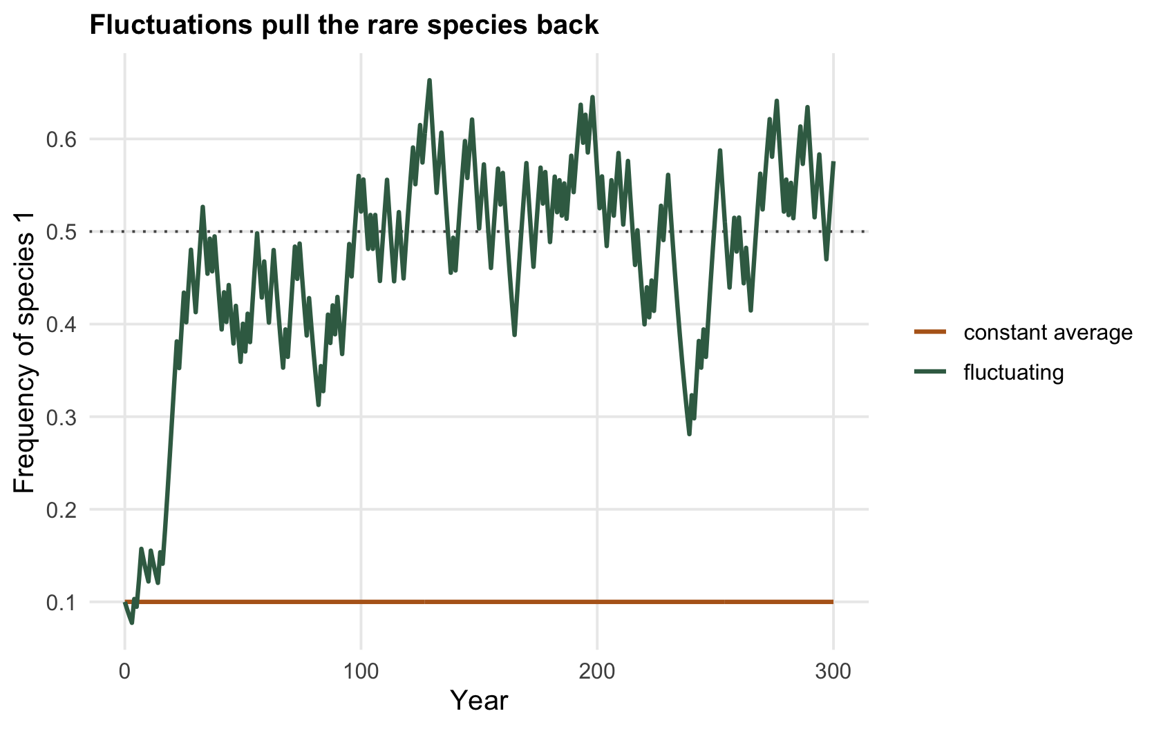
Start species 1 rare, at a frequency of 0.10. In the constant environment, where both species have the same average output, nothing pulls it back: it sits at 0.10, exactly where it started, because with equal outputs the recruit share equals the current frequency and there is no force at all. Turn the environment on and the rare species climbs back toward even, settling near 0.54. The fluctuation did what the constant environment could not: it gave the rare species a way back.

dt <- rbind(data.frame(t = 0:300, p = c_lo, env = "constant average"),
            data.frame(t = 0:300, p = f_lo, env = "fluctuating"))
ggplot(dt, aes(t, p, colour = env)) +
  geom_hline(yintercept = 0.5, colour = col_ref, linetype = "dotted") +
  geom_line(linewidth = 0.9) +
  scale_colour_manual(values = c("constant average" = col_const, "fluctuating" = col_fluc)) +
  labs(x = "Year", y = "Frequency of species 1", colour = NULL,
       title = "Fluctuations pull the rare species back")

Figure 1: Frequency of a species that starts rare, at 0.10. In the constant average environment (ochre) it stays put, no force acts on it; once the environment fluctuates (green) it is pulled back toward even, a stable coexistence.

Why the rare species gains

The reason is the rare-species advantage, and it comes from three ingredients that all have to be present. First, the species respond differently to the environment: a good year for one is not a good year for the other, so being rare means waiting for your own good years. Second, and this is the piece that gives the effect its name, the gains are stored. A rare species that has a bumper year does not have to cash the whole windfall at once and lose it in the next bad year; its long-lived adults carry the population through, storing the good year’s gain in a stage the environment cannot easily take back. Third, competition and the environment line up: a common species suffers its worst crowding exactly in its good years, when its own recruits flood the open sites, while a rare species in a good year meets little of its own kind and escapes that crowding. Put the invader rare and its long-run growth rate is positive.

inv_growth <- function(d) {
  # per-capita finite rate of a rare invader = (1-d) + d * (own output / resident output)
  mean(log(sapply(states, function(s) (1 - d) + d * s[1] / s[2])))
}
round(inv_growth(0.1), 3)

[1] 0.159

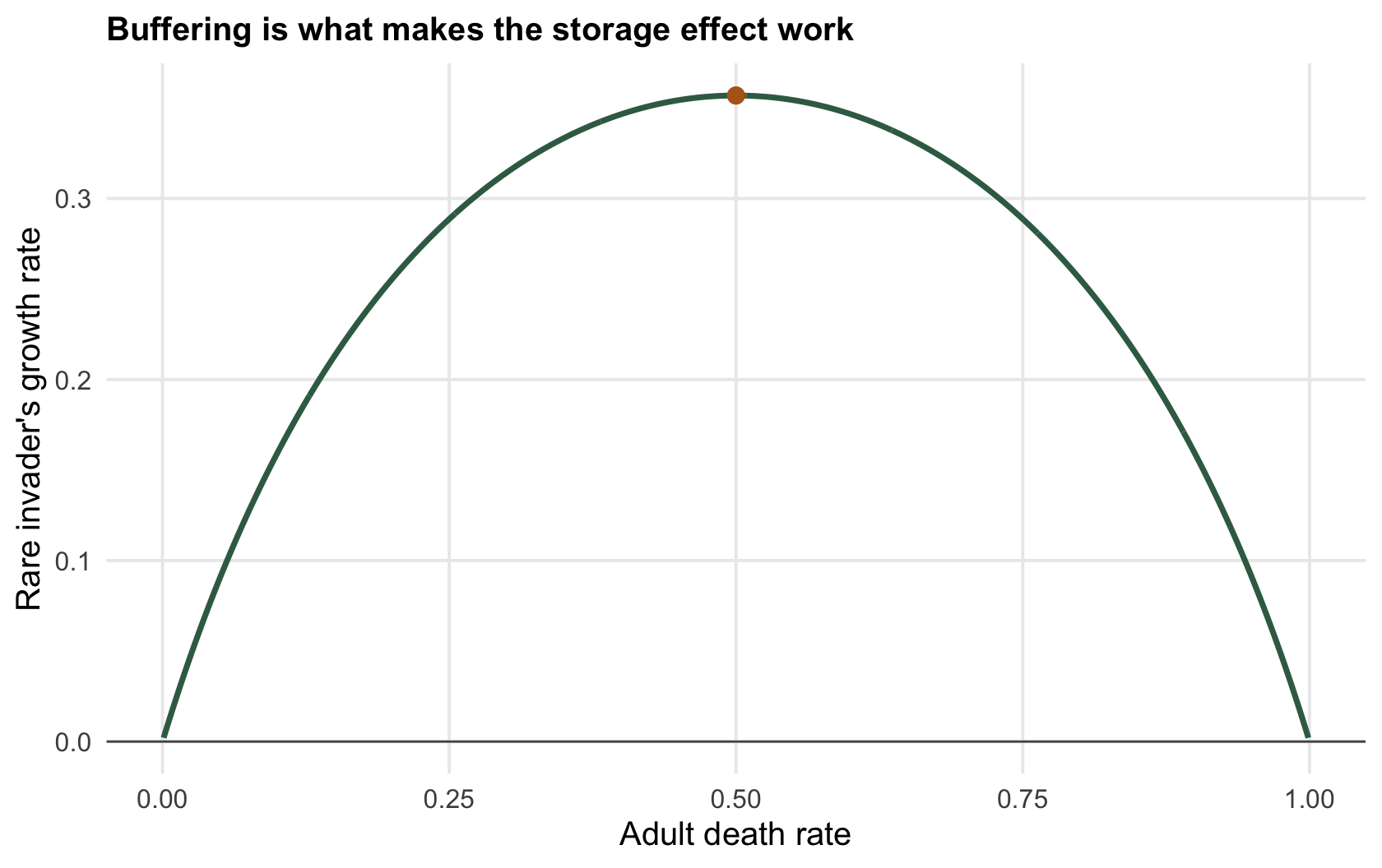
The rare invader grows at +0.159 per year on average, firmly positive, so it cannot be lost; and because the two species are mirror images, each invades the other and they coexist. The whole mechanism lives in the buffering. Adults must be long-lived enough to carry a good year forward: sweep the death rate from short-lived to fully annual and the invasion growth rate rises then falls, vanishing at both ends.

dd <- data.frame(delta = ds, r = rr)
ggplot(dd, aes(delta, r)) +
  geom_hline(yintercept = 0, colour = col_ref, linewidth = 0.4) +
  geom_line(colour = col_fluc, linewidth = 1) +
  annotate("point", x = d_peak, y = r_peak, colour = col_const, size = 2.4) +
  labs(x = "Adult death rate", y = "Rare invader's growth rate",
       title = "Buffering is what makes the storage effect work")

Figure 2: The rare invader’s growth rate against the adult death rate. It is zero when nothing turns over and zero again when generations do not overlap at all; the storage effect is strongest at intermediate longevity.

The peak sits at a death rate of 0.50, where the growth rate reaches +0.357. At the right-hand edge, a death rate of one, every adult dies each year and there is no overlap between generations, so nothing is stored and the advantage collapses to zero. Annual plants with no seed bank sit at exactly that edge, which is why the seed bank matters so much: it is the storage. At the left-hand edge almost nothing turns over, so the environmental signal barely enters and the rare species climbs back only slowly. The mechanism needs both turnover to feel the good years and buffering to keep them.

What the storage effect explains, and what it does not

The storage effect is attractive because it turns environmental variability, usually thought of as a threat to small populations, into something that actively maintains diversity. It offers an answer to old puzzles like the paradox of the plankton, where many species share a handful of limiting resources in a well-mixed water column that should permit only a few. But it is not a universal solvent. It requires genuine differences in how species respond to the environment, real buffering through a long-lived or dormant stage, and enough environmental variation to matter; take any one away and it disappears. It is one of two ways fluctuations can promote coexistence, the other being relative nonlinearity, and both are measured through the same test, the growth rate of a species when it is rare.

Related tutorials

• Relative nonlinearity of competition
• Partitioning the invasion growth rate
• Checking a storage-effect analysis
• Niche and fitness differences

References

• Chesson PL, Warner RR 1981. The American Naturalist 117(6):923-943 (10.1086/283778).
• Chesson P 2000. Annual Review of Ecology and Systematics 31:343-366 (10.1146/annurev.ecolsys.31.1.343).