Partitioning the invasion growth rate

Invasion growth in R: testing coexistence in a fluctuating environment and splitting a rare species’ growth into a fluctuation-free part and the storage effect.

Every coexistence claim, in a constant environment or a fluctuating one, comes down to a single test: can a species recover when it is rare? If each competitor, pushed to low density, has a positive long-run growth rate while the others sit at their usual abundances, then none can be lost and they coexist. This is the invasion criterion, and under a fluctuating environment it does something a point estimate cannot: it lets you take the rare species’ growth rate apart and see exactly how much of it the fluctuations are providing.

The invasion criterion, restated for a variable world

In the lottery model a rare invader’s per-capita growth in any year is its surviving adults plus the recruits it wins, which when it is rare depends on its own output relative to the resident’s. Averaged over the environmental states, its long-run growth rate is the mean of the log of that yearly factor. Compute it for a rare species, and compute the same thing for its competitor, to confirm each can invade the other.

delta <- 0.1
states <- list(c(3, 0.5), c(0.5, 3))                # negatively correlated outputs
inv_growth <- function(d, st = states) {
  mean(log(sapply(st, function(s) (1 - d) + d * s[1] / s[2])))
}
c(species1 = inv_growth(0.1), species2 = inv_growth(0.1))  # symmetric pair

 species1  species2 
0.1592269 0.1592269 

Both rare-invader growth rates come out at +0.159, positive, so each species invades a community of the other and the two coexist. That is the verdict. The interesting question is why the number is positive, and the way to answer it is to ask what the growth rate would be if the environment stopped fluctuating.

Splitting the growth rate

Freeze the environment at its average and recompute the invader’s growth. Whatever is left after you subtract that fluctuation-free value from the true, fluctuating one is the contribution the variability itself is making: the storage effect.

# fluctuation-free growth: environment held at its mean output for each species
mean_ratio <- mean(sapply(states, `[`, 1)) / mean(sapply(states, `[`, 2))
r_flat <- log((1 - delta) + delta * mean_ratio)
c(full = inv_growth(0.1), fluctuation_free = r_flat, storage_effect = inv_growth(0.1) - r_flat)

            full fluctuation_free   storage_effect 
       0.1592269        0.0000000        0.1592269 

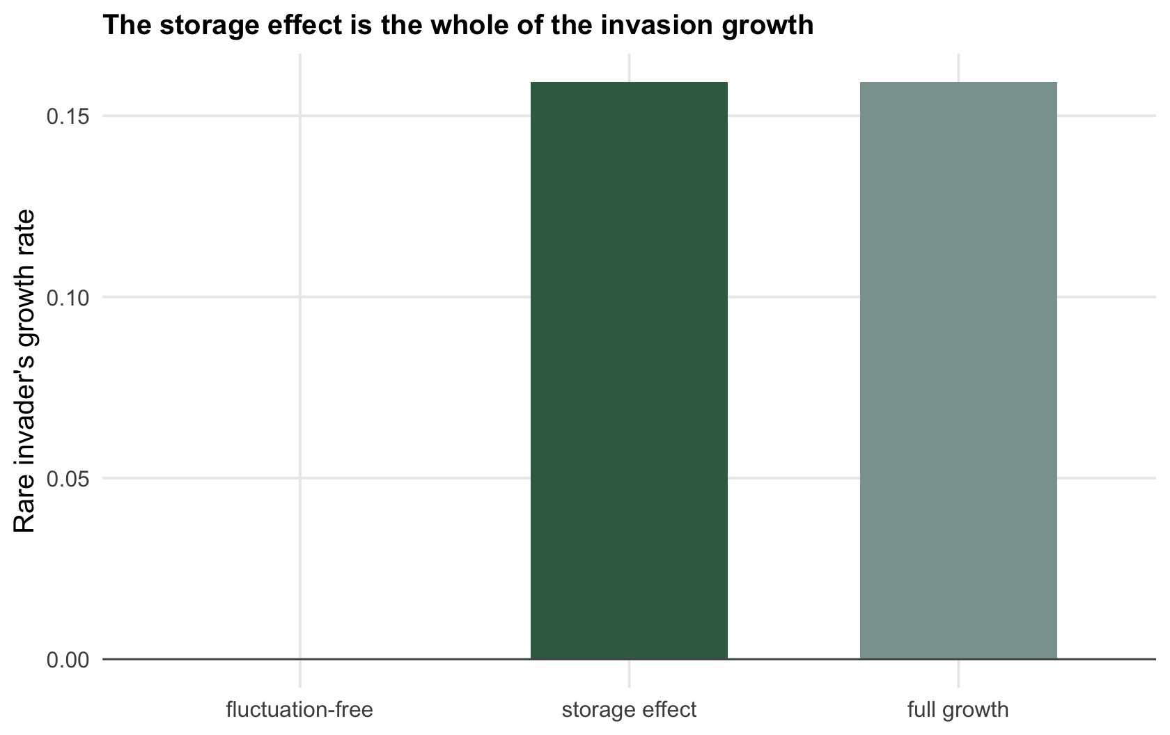
With the environment frozen at its mean the invader grows at 0.000, exactly zero: the two species are identical on average, so with no fluctuations neither has any advantage when rare, and the community is only neutrally stable. The entire +0.159 of real invasion growth is the storage effect. This is the partition that coexistence theory is built on: a rare species’ growth rate is a fluctuation-free part, which here contributes nothing, plus the fluctuation-dependent parts, which here contribute everything.

dp <- data.frame(part = factor(c("fluctuation-free", "storage effect", "full growth"),
                               levels = c("fluctuation-free", "storage effect", "full growth")),
                 val = c(r_flat, storage, r_full))
ggplot(dp, aes(part, val, fill = part)) +
  geom_col(width = 0.6) +
  geom_hline(yintercept = 0, colour = col_ref, linewidth = 0.4) +
  scale_fill_manual(values = c("fluctuation-free" = col_flat, "storage effect" = col_full,
                               "full growth" = col_alt), guide = "none") +
  labs(x = NULL, y = "Rare invader's growth rate",
       title = "The storage effect is the whole of the invasion growth")

Figure 1: The rare invader’s growth rate, split. Held at the mean environment (ochre) it is zero: no coexistence force. The fluctuations add the storage effect (green), which is the whole of the positive invasion growth.

Where the storage effect comes from: environment meets competition

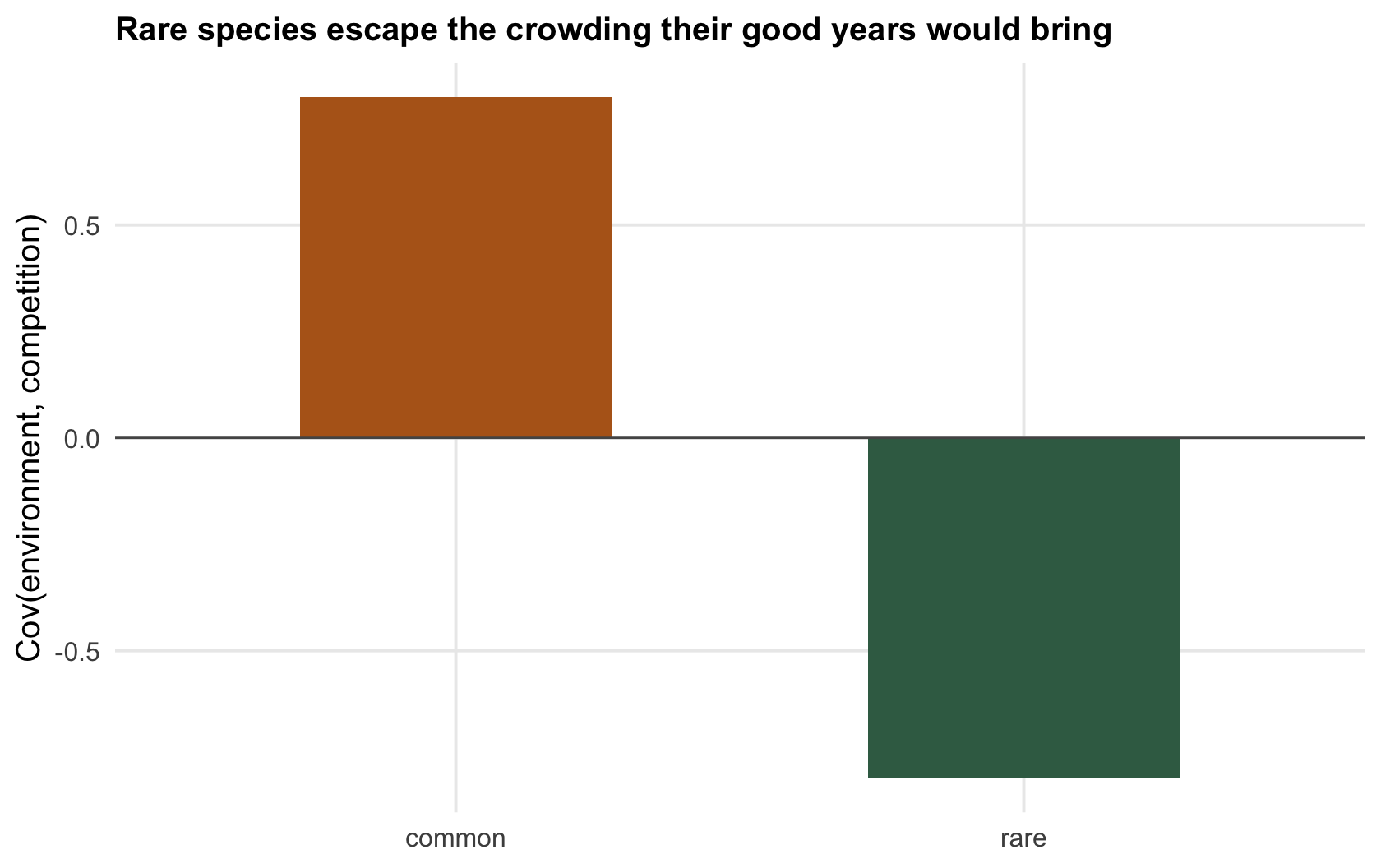
The storage effect is not magic arithmetic; it has a mechanism, and it is a covariance. Track two things for a focal species each year: its response to the environment, and the competition it experiences. When the species is common, its good years are exactly its most crowded years, because its own abundant recruits are the competition; environment and competition move together. When the species is rare, its good years are quiet, because it meets mostly the other species; the two decouple. Measure that covariance at low and high frequency.

covEC <- function(p) {
  E <- log(sapply(states, `[`, 1))                              # environmental response
  C <- log(sapply(states, function(s) s[1]*p + s[2]*(1 - p)))   # competition experienced
  mean(E*C) - mean(E)*mean(C)
}
c(rare = covEC(0.001), common = covEC(0.999))

      rare     common 
-0.7999929  0.7999929 

When the species is rare the covariance between its environment and its competition is -0.80, negative: in its good years it escapes competition. When common it is +0.80, positive: its good years are its most crowded. The rare-species advantage is precisely that difference. A rare species banks its good years without paying the crowding tax that the common species cannot avoid, and the buffering of long-lived adults is what lets it hold the gain. That is the storage effect stated in one line: coexistence comes from the environment and competition covarying less for the rare species than for the common one.

dc <- data.frame(state = c("rare", "common"), cov = c(cov_rare, cov_common))
ggplot(dc, aes(state, cov, fill = state)) +
  geom_col(width = 0.55) +
  geom_hline(yintercept = 0, colour = col_ref, linewidth = 0.4) +
  scale_fill_manual(values = c("rare" = col_full, "common" = col_flat), guide = "none") +
  labs(x = NULL, y = "Cov(environment, competition)",
       title = "Rare species escape the crowding their good years would bring")

Figure 2: Covariance between a species’ environmental response and the competition it feels, at low and high frequency. Rare (green) it is negative, good years are uncrowded; common (ochre) it is positive, good years are crowded. The gap is the rare-species advantage.

What the partition buys you

The value of splitting the growth rate is that it turns a yes-or-no coexistence result into an attribution. A positive invasion growth rate says the species coexist; the partition says whether they coexist because of stable differences that would survive in a constant world, or because of the fluctuations themselves, and if the latter, through which mechanism. That distinction matters for prediction: coexistence propped up by environmental variability is only as reliable as the variability, and a run of similar years, or a climate that dampens the swings, can dismantle it in a way that fluctuation-free coexistence would shrug off. The same partition extends to relative nonlinearity and to any number of species; the discipline of building it correctly, and the ways it misleads, are the checking post.

Related tutorials

• The storage effect and coexistence
• Relative nonlinearity of competition
• Checking a storage-effect analysis
• Rare-species advantage and coexistence

References

• Chesson P 2000. Annual Review of Ecology and Systematics 31:343-366 (10.1146/annurev.ecolsys.31.1.343).
• Chesson PL, Warner RR 1981. The American Naturalist 117(6):923-943 (10.1086/283778).