---
title: "Relative nonlinearity of competition"
description: "Relative nonlinearity in R: how curvature in a species' response to a fluctuating limiting factor becomes a second fluctuation-dependent route to coexistence."
date: "2026-07-04 11:00"
date-modified: "2026-10-15"
categories: [ecology tutorial, R, community ecology, coexistence, theoretical ecology]
image: thumbnail.png
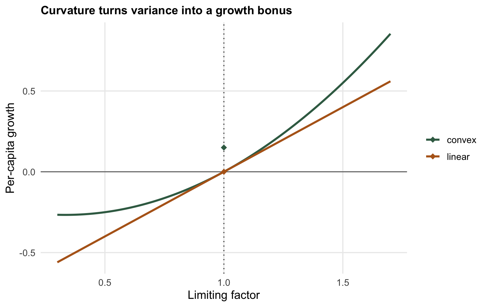
image-alt: "A convex growth curve and a straight one meeting at zero at the mean of the limiting factor, with the convex curve above the straight one on both sides and the average of the convex response under fluctuation marked above zero, the Jensen gap that relative nonlinearity exploits."
---
*Corrected 15 October 2026: the post gave the condition that the species profiting from fluctuation must damp it as the one condition for coexistence; it now says that condition is needed but not enough, and that the linear species of this pair cannot invade a convex resident unless it also has an edge at constant conditions.*
*Corrected 7 October 2026: the post said a curvature difference alone can let two species coexist, credited Jensen's inequality with the size of the growth bonus, and titled the invasion figure as fluctuations letting the convex species in; it now adds the condition that the species profiting from fluctuation must damp it, says Jensen's inequality gives only the sign while the half-curvature-times-variance formula is exact for this quadratic response, and titles the figure as a growth bonus under imposed fluctuation.*
*Corrected 30 September 2026: the post said the invasion calculation had opened a route in for a species that would otherwise be shut out; it now says the calculation shows a growth bonus for the convex species under imposed fluctuation, which is only one half of a coexistence argument.*
```{r setup}
#| code-fold: true
#| code-summary: "Setup: packages, colours and plot theme"
#| results: hide
#| message: false
#| warning: false
knitr::opts_chunk$set(echo = TRUE, message = FALSE, warning = FALSE,
                      dev = "png", dpi = 120, fig.path = "figures/",
                      fig.width = 7, fig.height = 4.4)
library(ggplot2)
theme_te <- theme_minimal(base_size = 12) +
  theme(panel.background = element_rect(fill = "#f5f4ee", colour = NA),
        plot.background  = element_rect(fill = "#f5f4ee", colour = NA),
        panel.grid.minor = element_blank(),
        plot.title = element_text(face = "bold", size = 12))
theme_set(theme_te)
col_lin <- "#b5651d"; col_con <- "#3a6b52"; col_ref <- "#555555"

Rstates <- c(0.5, 1.5)              # fluctuating limiting factor, mean 1
Rbar <- mean(Rstates)
gL <- function(R) 0.8*R - 0.8                     # linear responder
gV <- function(R) 0.8*R + 0.6*(R - 1)^2 - 0.8     # convex responder, same value and slope at the mean
EL <- mean(sapply(Rstates, gL)); EV <- mean(sapply(Rstates, gV))
gLbar <- gL(Rbar); gVbar <- gV(Rbar)
gpp <- 1.2                                        # second derivative of the convex responder
varR <- mean((Rstates - Rbar)^2)
jensen <- 0.5 * gpp * varR
```
The [storage effect](../the-storage-effect/) is one way a fluctuating environment can hold competitors together. There is a second, and it is easy to miss because it hides inside a piece of school algebra: the average of a curved function is not the function of the average. When two species differ in how curved their response to a fluctuating limiting factor is, that difference can let them coexist, provided the species that profits from the fluctuation is the one that damps it when common and the other species has an edge at constant conditions of the right size. This is relative nonlinearity, the subtler of the two fluctuation-dependent mechanisms.
## Jensen's inequality, made ecological
Suppose a species' per-capita growth depends on some fluctuating quantity: a shared resource, the intensity of competition, a limiting factor that rises and falls from year to year. If that dependence is a straight line, fluctuations wash out: the good years and the bad years cancel, and the average growth is exactly the growth at the average condition. If the dependence *curves upward*, they do not cancel. The species gains more in the good years than it loses in the bad, so fluctuations lift its average growth above the constant-environment value. That is Jensen's inequality, and the gap it opens is the engine here.
```{r jensen}
Rstates <- c(0.5, 1.5)                             # limiting factor swings around a mean of 1
gL <- function(R) 0.8*R - 0.8                      # linear response: no curvature
gV <- function(R) 0.8*R + 0.6*(R - 1)^2 - 0.8      # convex response: curves upward
# at the mean condition the two species are identical; compare their averages under fluctuation
c(linear_mean   = mean(sapply(Rstates, gL)),
  convex_mean   = mean(sapply(Rstates, gV)),
  linear_atmean = gL(1), convex_atmean = gV(1))
```
The two species are built to be identical at the average condition: both have growth `r sprintf("%.2f", gLbar)` when the limiting factor sits at its mean. Under fluctuation they part company. The linear species averages `r sprintf("%.3f", EL)`, unchanged, because a straight line has nothing to exploit. The convex species averages `r sprintf("%+.3f", EV)`, lifted above zero purely by the variance. The size of that lift is set by the curvature and the variance together. Jensen's inequality gives only its sign; for a quadratic response like this one the lift is exactly half the second derivative times the variance, and for other smooth curves that formula is a second-order approximation.
```{r jensen-check}
gpp <- 1.2                                         # second derivative of the convex responder
varR <- mean((Rstates - 1)^2)                      # variance of the limiting factor
c(realised_gain = mean(sapply(Rstates, gV)) - gV(1),
  curvature_formula = 0.5 * gpp * varR)
```
The realised gain and the prediction agree at `r sprintf("%+.3f", jensen)`: the convex species' bonus is exactly half its curvature times the variance of the limiting factor. Nothing about this depended on the mean; two species with identical average responses can have completely different average *growth* once the environment varies, as long as their curvatures differ.
```{r fig-jensen}
#| fig-cap: "Growth against a fluctuating limiting factor. Both responses pass through zero at the mean (dotted). Averaging over the two environmental states leaves the linear species at zero but lifts the convex species above it, the Jensen gap."
#| fig-alt: "Two growth curves against a limiting factor, one straight and one curving upward, both through zero at the mean; markers show the averaged convex value sits above zero while the linear average stays at zero."
rg <- seq(0.3, 1.7, 0.01)
dl <- rbind(data.frame(R = rg, g = sapply(rg, gL), sp = "linear"),
            data.frame(R = rg, g = sapply(rg, gV), sp = "convex"))
pts <- data.frame(R = 1, g = c(EL, EV), sp = c("linear", "convex"))
ggplot(dl, aes(R, g, colour = sp)) +
  geom_hline(yintercept = 0, colour = col_ref, linewidth = 0.4) +
  geom_vline(xintercept = 1, colour = col_ref, linetype = "dotted") +
  geom_line(linewidth = 1) +
  geom_point(data = pts, aes(R, g, colour = sp), size = 2.6, shape = 18) +
  scale_colour_manual(values = c("linear" = col_lin, "convex" = col_con)) +
  labs(x = "Limiting factor", y = "Per-capita growth", colour = NULL,
       title = "Curvature turns variance into a growth bonus")
```
## From a bonus to coexistence
A growth bonus is not yet coexistence; coexistence needs each species to gain when it is rare. Relative nonlinearity can deliver that only under a condition worth stating plainly: the species that profits from variance in the limiting factor has to be the species that damps it. When that holds, the convex, variance-loving species sits, while rare, in an environment made variable by its competitor and reaps the Jensen bonus; once common, it flattens that variance itself and gives the bonus up. That condition is needed but not enough, because the linear species must gain when rare too, and for the pair here it cannot: the linear response is the convex one minus a squared term, so a convex resident whose average growth is zero leaves the linear invader with negative average growth whenever the limiting factor still varies at all. To coexist, the linear species would also need an edge at constant conditions, big enough to outweigh whatever bonus the convex species still draws from the variance it leaves when common, and small enough that the convex species can still invade. Run the invasion test at the mean condition and under fluctuation.
```{r invasion}
# invader growth when the limiting factor is held constant vs when it fluctuates
c(constant_linear = gL(1), constant_convex = gV(1),
  fluct_linear = mean(sapply(Rstates, gL)), fluct_convex = mean(sapply(Rstates, gV)))
```
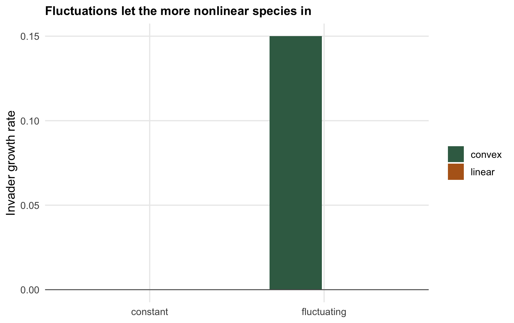
Held constant, both invaders sit at `r sprintf("%.2f", gVbar)`: a dead heat, no mechanism, and the slightest average difference would decide the whole community. Let the factor fluctuate and the convex species invades at `r sprintf("%+.3f", EV)` while the linear species stays at `r sprintf("%.3f", EL)`. The curvature difference, and nothing else, gives the convex species a positive growth rate under this imposed fluctuation. That is one half of a coexistence argument only: the linear species still sits at zero, and a full invasion test would let the variance of the limiting factor depend on which species is common, which this calculation does not do. For this pair that fuller test would put the linear species below zero, as argued above, unless it also had an edge at constant conditions.
```{r fig-invasion}
#| fig-cap: "Invader growth for the two species. In a constant environment both are tied at zero, no coexistence force; once the limiting factor fluctuates the convex, variance-loving species gains a positive growth rate while the linear one does not."
#| fig-alt: "A grouped bar chart of invader growth for a linear and a convex species under a constant and a fluctuating environment; only the convex species under fluctuation rises above zero."
di <- rbind(data.frame(sp = "linear", env = "constant",    r = gLbar),
            data.frame(sp = "convex", env = "constant",    r = gVbar),
            data.frame(sp = "linear", env = "fluctuating", r = EL),
            data.frame(sp = "convex", env = "fluctuating", r = EV))
di$env <- factor(di$env, levels = c("constant", "fluctuating"))
ggplot(di, aes(env, r, fill = sp)) +
  geom_col(position = position_dodge(width = 0.65), width = 0.6) +
  geom_hline(yintercept = 0, colour = col_ref, linewidth = 0.4) +
  scale_fill_manual(values = c("linear" = col_lin, "convex" = col_con)) +
  labs(x = NULL, y = "Invader growth rate", fill = NULL,
       title = "Imposed fluctuation gives the convex invader a growth bonus")
```
## The honest boundary
Relative nonlinearity is real but it is delicate, and it deserves more caveats than the storage effect. The sign of the effect depends on which species has the more convex response *and* on which species generates more variance in the limiting factor, and these can point the same way or opposite ways; relative nonlinearity can just as easily *destabilise* a pair as stabilise it. It usually produces a weaker coexistence than the storage effect, and in models with a single fluctuating resource it often needs the fluctuations to be self-generated, through consumer-resource cycles, rather than imposed from outside. The lesson to carry is narrow and solid: curvature plus variance changes average growth, two species that differ in curvature therefore differ in how fluctuations treat them, and that difference is a coexistence mechanism in its own right. Whether it helps or hurts a particular pair is a question the [invasion growth rate](../partitioning-invasion-growth/) has to answer case by case.
## References
- Chesson P 2000. Annual Review of Ecology and Systematics 31:343-366 (10.1146/annurev.ecolsys.31.1.343).
- Armstrong RA, McGehee R 1980. The American Naturalist 115(2):151-170 (10.1086/283553).
## Related tutorials
- [The storage effect and coexistence](../the-storage-effect/)
- [Partitioning the invasion growth rate](../partitioning-invasion-growth/)
- [Checking a storage-effect analysis](../checking-a-storage-effect-analysis/)
- [Stochastic population growth](../stochastic-population-growth/)