How many visits? Occupancy survey design

Decide how many repeat visits an occupancy survey needs, from cumulative detection to the sites-versus-visits trade-off under a fixed budget, worked in R.

Every occupancy survey faces the same two questions before a single site is visited. How many times should each site be visited, so that a non-detection carries real weight? And given a fixed amount of fieldwork, is it better to visit many sites a few times or few sites many times? The first question is about confidence in a single blank; the second is about the precision of the occupancy estimate as a whole. Both have clean answers, and neither needs a simulation to see the shape.

When does a blank mean something?

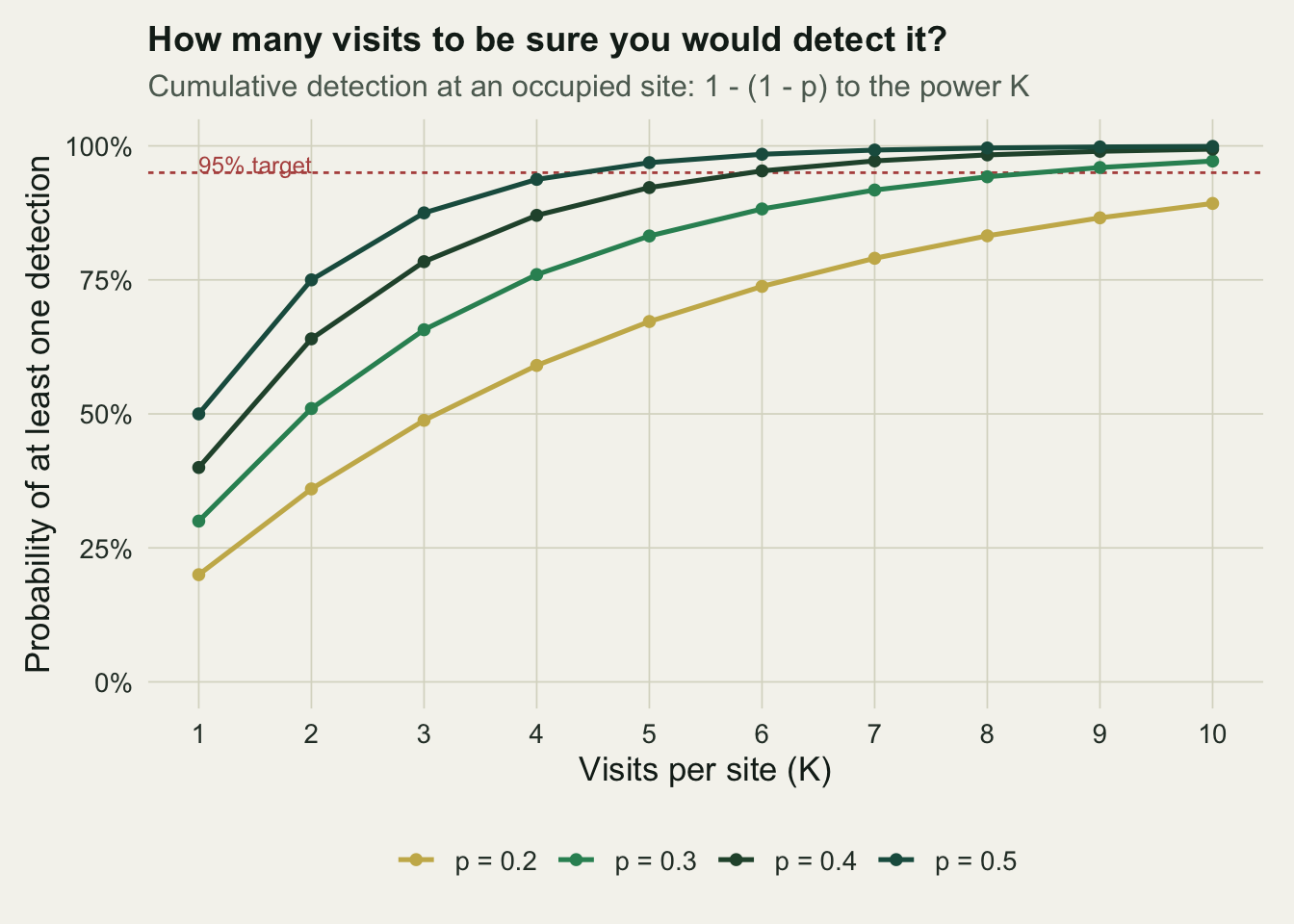
An occupied site yields at least one detection across K visits with probability 1 - (1 - p)^K, the same expression that drove the detection-bias tutorial. Read as a design tool, it says how many visits you need before a run of blanks is good evidence of absence. If a species is easy to detect, a couple of visits suffice; if it is cryptic, a blank stays ambiguous for a long time.

K_seq <- 1:10; ps <- c(0.2, 0.3, 0.4, 0.5)
cd <- expand.grid(K = K_seq, p = ps)
cd$cum <- 1 - (1 - cd$p)^cd$K
cd$plab <- factor(sprintf("p = %.1f", cd$p))
ggplot(cd, aes(K, cum, colour = plab)) +
  geom_hline(yintercept = 0.95, colour = te_red, linewidth = 0.5, linetype = "22") +
  annotate("text", x = 1, y = 0.965, label = "95% target", hjust = 0, colour = te_red, size = 3.2) +
  geom_line(linewidth = 0.9) + geom_point(size = 1.6) +
  scale_colour_manual(values = c("p = 0.2"=te_gold, "p = 0.3"=te_green,
                                 "p = 0.4"=te_forest, "p = 0.5"=te_deep), name = NULL) +
  scale_x_continuous(breaks = 1:10) +
  scale_y_continuous(limits = c(0, 1), labels = scales::percent_format(1)) +
  labs(title = "How many visits to be sure you would detect it?",
       subtitle = "Cumulative detection at an occupied site: 1 - (1 - p) to the power K",
       x = "Visits per site (K)", y = "Probability of at least one detection") +
  theme_te(13)

Figure 1: Cumulative probability of at least one detection at an occupied site, against visits per site, for four detection probabilities. The dashed line marks a 95 per cent target.

The visits needed to reach a chosen level of confidence follow from solving 1 - (1 - p)^K = 0.95 for K, which gives K = log(0.05) / log(1 - p), rounded up.

p_grid <- c(0.15, 0.20, 0.30, 0.40, 0.50)
data.frame(p = p_grid,
           visits_for_95 = ceiling(log(0.05) / log(1 - p_grid)))

     p visits_for_95
1 0.15            19
2 0.20            14
3 0.30             9
4 0.40             6
5 0.50             5

A readily detected species with p = 0.5 reaches 95 per cent confidence in five visits, but a cryptic one with p = 0.15 needs nineteen. This is the false-absence problem stated as a budget: with too few visits, a string of blanks at an occupied site is common, and any analysis that reads those blanks as absences inherits the error. It also connects back to the earlier detection-bias example, where p = 0.3 and four visits gave a cumulative detection of 1 - 0.7^4, about 0.760, which is well short of certainty and explains why a quarter of occupied sites there went unrecorded.

A fixed budget: more sites or more visits?

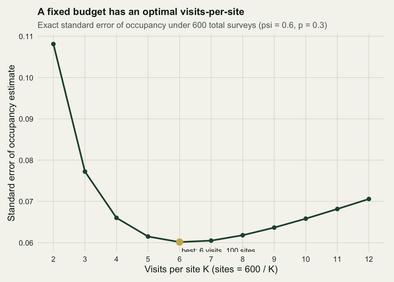
Confidence in a single blank is only half the design. The other half is the precision of the occupancy estimate itself, and here more visits per site compete against more sites. Suppose the total fieldwork is fixed at 600 site-visits. You could survey 300 sites twice, 100 sites six times, or 60 sites ten times. Each split spends the same effort but estimates occupancy with a different standard error.

The precision can be computed exactly, without simulating, from the Fisher information of the single-season likelihood. For a given psi and p, each visit history d from 0 to K occurs with a known probability, and each carries a score for psi and for p. Summing the outer products of those scores, weighted by their probabilities, gives the per-site information matrix; inverting it and dividing by the number of sites gives the variance of the occupancy estimate.

asymp_se_psi <- function(psi, p, K, R) {
  d  <- 0:K
  Pd <- ifelse(d >= 1, psi * choose(K, d) * p^d * (1 - p)^(K - d),
               psi * (1 - p)^K + (1 - psi))
  A0 <- psi * (1 - p)^K + (1 - psi)
  s_psi <- ifelse(d >= 1, 1 / psi, ((1 - p)^K - 1) / A0)
  s_p   <- ifelse(d >= 1, d / p - (K - d) / (1 - p), psi * (-K) * (1 - p)^(K - 1) / A0)
  I <- matrix(c(sum(Pd * s_psi^2), sum(Pd * s_psi * s_p),
                sum(Pd * s_psi * s_p), sum(Pd * s_p^2)), 2, 2)
  sqrt(solve(I)[1, 1] / R)
}

With psi = 0.6, p = 0.3 and a budget of 600 site-visits, we sweep the number of visits from two to twelve, letting the number of sites fall as visits rise.

B <- 600; psi0 <- 0.6; p0 <- 0.3
dd <- data.frame(K = 2:12)
dd$R  <- B / dd$K
dd$se <- mapply(function(k, r) asymp_se_psi(psi0, p0, k, r), dd$K, dd$R)
kmin <- dd$K[which.min(dd$se)]
ggplot(dd, aes(K, se)) +
  geom_line(colour = te_forest, linewidth = 1) +
  geom_point(size = 2, colour = te_forest) +
  geom_point(data = subset(dd, K == kmin), colour = te_gold, size = 3.6) +
  annotate("text", x = kmin, y = min(dd$se),
           label = sprintf(" best: %d visits, %d sites", kmin, B / kmin),
           hjust = 0, vjust = 2.1, colour = te_ink, size = 3.3) +
  scale_x_continuous(breaks = 2:12) +
  labs(title = "A fixed budget has an optimal visits-per-site",
       subtitle = "Exact standard error of occupancy under 600 total surveys (psi = 0.6, p = 0.3)",
       x = "Visits per site K (sites = 600 / K)", y = "Standard error of occupancy estimate") +
  theme_te(12)

Figure 2: Exact standard error of the occupancy estimate against visits per site, under a fixed budget of 600 site-visits. The gold point marks the best split.

dd$se <- round(dd$se, 4)
dd[, c("K", "R", "se")]

    K         R     se
1   2 300.00000 0.1081
2   3 200.00000 0.0772
3   4 150.00000 0.0660
4   5 120.00000 0.0615
5   6 100.00000 0.0601
6   7  85.71429 0.0605
7   8  75.00000 0.0618
8   9  66.66667 0.0637
9  10  60.00000 0.0658
10 11  54.54545 0.0682
11 12  50.00000 0.0706

Two visits to 300 sites is the worst of the options on offer, with a standard error of 0.108, because two visits leave detection too poorly estimated and the all-blank sites too ambiguous. Precision improves sharply as visits rise, reaches its best near six visits to 100 sites at a standard error of 0.060, then drifts back up as the shrinking pool of sites starts to cost more than the extra visits buy. Past the optimum you are paying to confirm detection at sites you already understand, while the estimate of how widespread the species is thins out.

The basin, not the point

The useful message is not the single best split but the shape around it. The curve is flat across roughly five to eight visits, so any split in that range spends the budget about as well as the optimum. The penalty for missing the exact minimum is small; the penalty for the extremes is large. Two visits is genuinely bad, and so, at the other end, is piling ten visits onto sixty sites.

Where the optimum sits depends on the truth you are planning around. Rare species, with low psi, and cryptic ones, with low p, both push the optimum towards more visits per site, because both make detection the binding constraint. That is why a pilot season matters: a rough estimate of p turns this curve from an abstraction into a concrete recommendation for how to spend next year’s effort. As a rule of thumb from the design literature, a handful of visits, often in the region of three to five for a moderately detectable species, and more for a cryptic one, spends a fixed budget close to as well as any split can.

References

• MacKenzie D I, Royle J A 2005 Journal of Applied Ecology 42(6):1105-1114 (10.1111/j.1365-2664.2005.01098.x)
• Guillera-Arroita G, Ridout M S, Morgan B J T 2010 Methods in Ecology and Evolution 1(2):131-139 (10.1111/j.2041-210X.2010.00017.x)
• Bailey L L, Hines J E, Nichols J D, MacKenzie D I 2007 Ecological Applications 17(1):281-290 (10.1890/1051-0761(2007)017[0281:SDTIOS]2.0.CO;2)

Related tutorials

• Fitting single-season occupancy models in R
• Imperfect detection and occupancy bias in R
• Power analysis by simulation in R
• Occupancy and detection covariates in R