sim_track <- function(n, gamma, sigma, tau, seed){
  set.seed(seed)
  vx <- numeric(n); vy <- numeric(n)
  vx[1] <- rnorm(1, 0, sigma/sqrt(1-gamma^2))   # stationary start
  vy[1] <- rnorm(1, 0, sigma/sqrt(1-gamma^2))
  for(t in 2:n){
    vx[t] <- gamma*vx[t-1] + rnorm(1,0,sigma)
    vy[t] <- gamma*vy[t-1] + rnorm(1,0,sigma)
  }
  px <- cumsum(vx); py <- cumsum(vy)
  ox <- px + rnorm(n,0,tau); oy <- py + rnorm(n,0,tau)
  list(px=px, py=py, ox=ox, oy=oy)
}
n <- 400; gamma_t <- 0.7; sigma_t <- 4; tau_t <- 6
tr <- sim_track(n, gamma_t, sigma_t, tau_t, seed=6041)State-space models for animal movement
movement ecology
state-space models
Kalman filter
time series
R
ecology tutorial
Fit a linear-Gaussian correlated random walk to noisy telemetry in base R: a hand-coded Kalman filter and smoother that separate real movement from observation error.
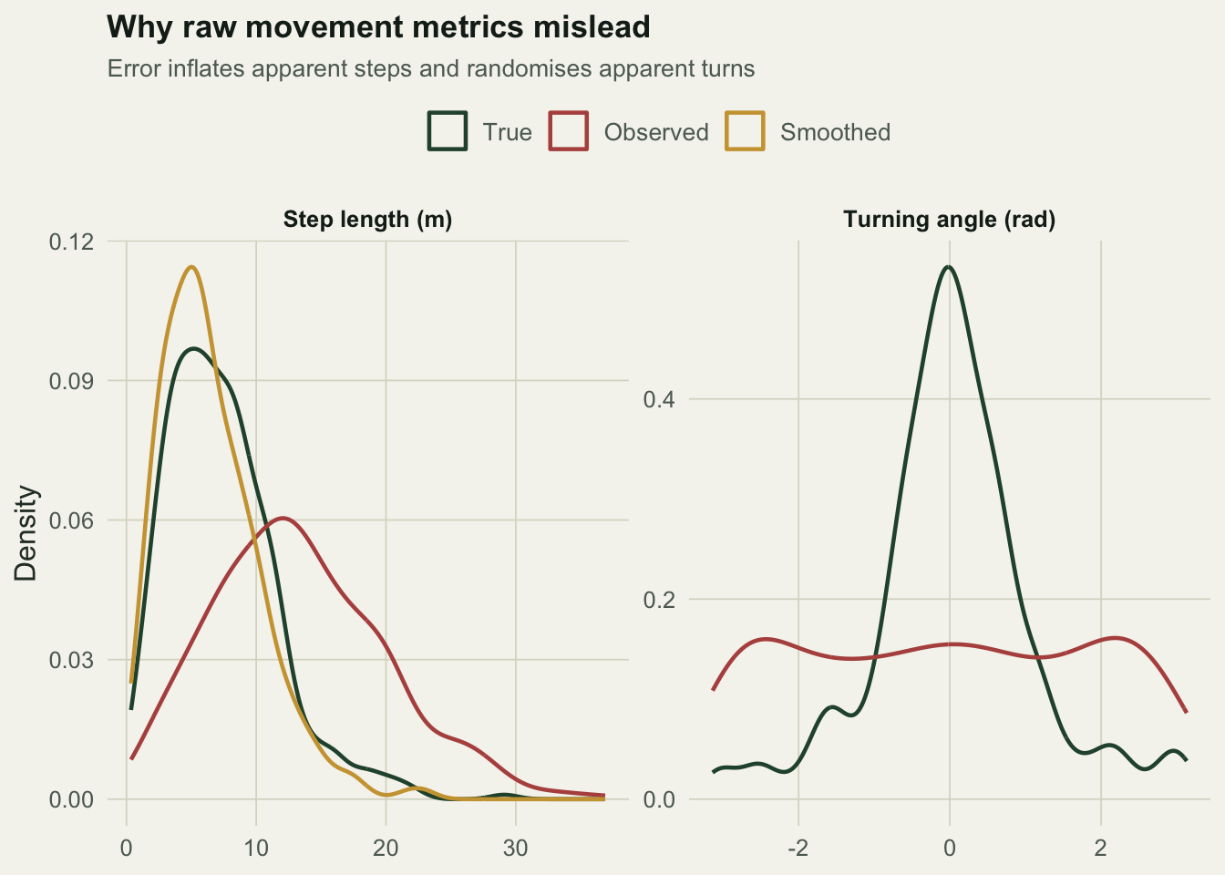
A GPS or Argos track is never the animal’s true path. Every fix carries location error, and that error does something worse than blur the picture: it systematically distorts the summaries we care about. Measured step lengths come out too long, and measured turning angles look far more random than the animal actually moved. A state-space model fixes this by treating the true positions as a hidden process observed through noise, then estimating both layers at once. This post builds the simplest useful version, a linear-Gaussian correlated random walk, with a Kalman filter and smoother coded by hand in base R.
The two-layer model
We split the problem into a movement process and an observation process. For each coordinate the animal has a velocity that persists from step to step, and a position that accumulates that velocity:
\[v_t = \gamma\, v_{t-1} + \varepsilon_t, \qquad p_t = p_{t-1} + v_t, \qquad \varepsilon_t \sim N(0, \sigma^2).\]
The persistence \(\gamma\) between 0 and 1 is directional autocorrelation: the same quantity a correlated random walk encodes. We then observe the position with additive Gaussian error:
\[y_t = p_t + \eta_t, \qquad \eta_t \sim N(0, \tau^2).\]
The state is the pair (position, velocity), which makes this a linear Gaussian state-space model. Written that way, the Kalman filter gives the exact likelihood, and the Rauch-Tung-Striebel smoother gives the best estimate of every position given the whole track.
Simulating a track we can check against
To know whether the method recovers the truth, we simulate a track with known parameters and then hide it behind observation error. A velocity persistence of 0.7, a process standard deviation of 4 metres, and an observation standard deviation of 6 metres give a realistic level of noise for a fine-scale tag.
The Kalman filter, by hand
The filter walks forward through the track. At each step it predicts the next state from the movement model, compares the prediction with the observation, and corrects. The by-products are the one-step prediction error and its variance, which multiply together into the Gaussian log-likelihood. We condition on the first observation to start the recursion cleanly.
kf_coord <- function(y, g, s2, h2){
  n <- length(y)
  Tm <- matrix(c(1,0, g,g), 2,2)          # rows: (1, g), (0, g)
  Q  <- s2*matrix(c(1,1,1,1),2,2)
  Z  <- matrix(c(1,0),1,2)
  a  <- c(y[1], 0)                         # condition on first fix
  P  <- matrix(c(h2,0,0, s2/(1-g^2)),2,2)
  ll <- 0
  af <- matrix(NA,n,2); Pf <- vector("list",n)
  ap <- matrix(NA,n,2); Pp <- vector("list",n)
  af[1,]<-a; Pf[[1]]<-P; ap[1,]<-a; Pp[[1]]<-P
  for(t in 2:n){
    ap_t <- as.vector(Tm %*% a)
    Pp_t <- Tm %*% P %*% t(Tm) + Q
    v  <- y[t] - as.vector(Z %*% ap_t)     # prediction error (innovation)
    Ft <- as.vector(Z %*% Pp_t %*% t(Z)) + h2
    K  <- as.vector(Pp_t %*% t(Z)) / Ft    # Kalman gain
    a  <- ap_t + K*v
    P  <- Pp_t - (K %*% Z) %*% Pp_t
    ll <- ll - 0.5*(log(2*pi)+log(Ft)+v^2/Ft)
    af[t,]<-a; Pf[[t]]<-P; ap[t,]<-ap_t; Pp[[t]]<-Pp_t
  }
  list(ll=ll, af=af, Pf=Pf, ap=ap, Pp=Pp, Tm=Tm)
}

rts <- function(fk){                        # Rauch-Tung-Striebel smoother
  n <- nrow(fk$af); Tm <- fk$Tm
  as <- fk$af; Ps <- fk$Pf
  for(t in (n-1):1){
    Pp1 <- fk$Pp[[t+1]]
    C <- fk$Pf[[t]] %*% t(Tm) %*% solve(Pp1)
    as[t,] <- fk$af[t,] + as.vector(C %*% (as[t+1,]-fk$ap[t+1,]))
    Ps[[t]] <- fk$Pf[[t]] + C %*% (Ps[[t+1]]-Pp1) %*% t(C)
  }
  list(as=as, Ps=Ps)
}
Estimating the parameters
The two coordinates are independent given the parameters, so their log-likelihoods add. We optimise on an unconstrained scale, mapping \(\gamma\) through a logistic link and the two variances through logs, so the optimiser never proposes an impossible value.
nll <- function(par, ox, oy){
  g <- plogis(par[1]); s2 <- exp(par[2]); h2 <- exp(par[3])
  -(kf_coord(ox,g,s2,h2)$ll + kf_coord(oy,g,s2,h2)$ll)
}
start <- c(qlogis(0.5), log(var(diff(tr$ox))/2), log(var(diff(tr$ox))/2))
fit <- optim(start, nll, ox=tr$ox, oy=tr$oy, method="Nelder-Mead",
             control=list(maxit=2000, reltol=1e-10))
g_hat   <- plogis(fit$par[1])
sig_hat <- sqrt(exp(fit$par[2]))
tau_hat <- sqrt(exp(fit$par[3]))
c(gamma=round(g_hat,3), sigma=round(sig_hat,3), tau=round(tau_hat,3))
gamma sigma tau
0.707 4.269 6.069 The estimates land close to the truth: persistence 0.707 against a true 0.7, process standard deviation 4.269 against 4, and observation standard deviation 6.069 against 6. The model has pulled apart two sources of variation that the raw track hopelessly confounds.
fkx <- kf_coord(tr$ox, g_hat, sig_hat^2, tau_hat^2); smx <- rts(fkx)
fky <- kf_coord(tr$oy, g_hat, sig_hat^2, tau_hat^2); smy <- rts(fky)
sx <- smx$as[,1]; sy <- smy$as[,1]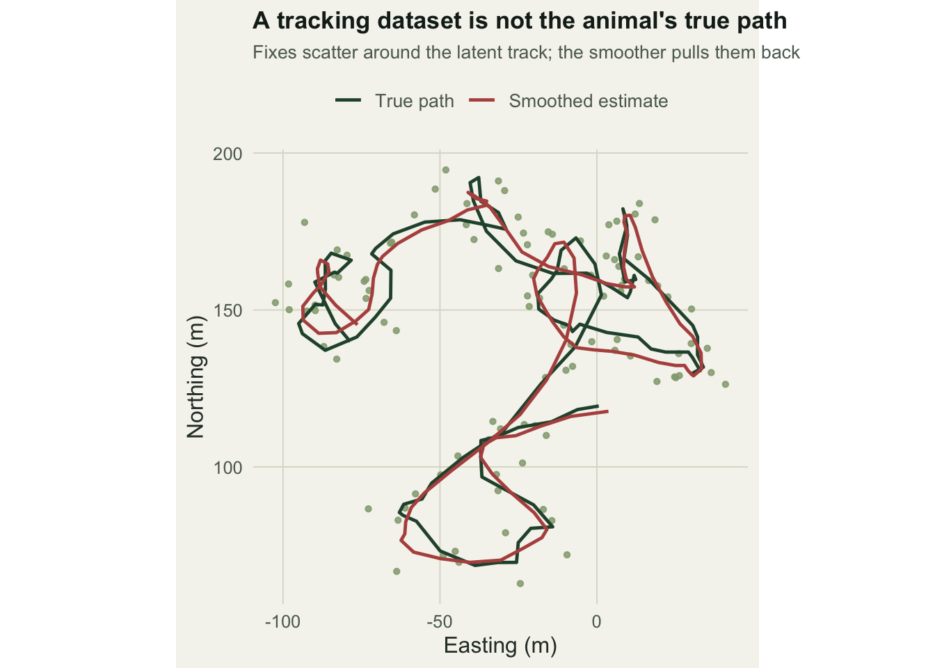
What the error does to movement metrics
Now the pay-off. Compute the total path length and the mean resultant length of the turning angles (a measure of directional concentration between 0 and 1) three ways: from the true path, from the raw observations, and from the smoothed estimate.
plen <- function(x,y) sum(sqrt(diff(x)^2+diff(y)^2))
turn_Rbar <- function(x,y){
  h <- atan2(diff(y),diff(x))
  ta <- diff(h); ta <- atan2(sin(ta),cos(ta))
  abs(mean(exp(1i*ta)))
}
pl_true <- plen(tr$px,tr$py); pl_obs <- plen(tr$ox,tr$oy); pl_sm <- plen(sx,sy)
Rb_true <- turn_Rbar(tr$px,tr$py); Rb_obs <- turn_Rbar(tr$ox,tr$oy); Rb_sm <- turn_Rbar(sx,sy)
rmse <- function(ex,ey) sqrt(mean((ex-tr$px)^2+(ey-tr$py)^2))
rmse_obs <- rmse(tr$ox,tr$oy); rmse_sm <- rmse(sx,sy)
The true path is 2918 metres long. The raw observations trace 5301 metres, an inflation of 1.82 times, because the error adds a spurious zig-zag to every segment. The smoothed path comes to 2578 metres. Turning angles tell the same story in reverse: the true resultant length is 0.612 (a fairly directed walk), but the observations give 0.07, close to zero, making the animal look as though it turned at random. The smoother restores directional structure, to 0.798. Measured against the true positions, the raw fixes sit 8.59 metres away on average, and the smoother roughly halves that to 4.96 metres.
Where this can go wrong
The smoother is not magic. It over-smooths a little here, nudging the turning-angle concentration slightly above the truth, because with a single track the estimated observation error absorbs some genuine movement. That trade-off is the central difficulty of these models. When the observation error is large relative to the movement between fixes, or the track is short, the process and observation variances become hard to separate, and estimates drift. The companion posts on regularising irregular tracks and on model checking take that problem head-on. The lesson to carry forward is simple: never compute path length or tortuosity from a raw track without first accounting for the error in the fixes.
References
Jonsen, Flemming and Myers 2005. Ecology 86(11):2874-2880 (10.1890/04-1852)
Morales, Haydon, Frair, Holsinger and Fryxell 2004. Ecology 85(9):2436-2445 (10.1890/03-0269)
Patterson, Thomas, Wilcox, Ovaskainen and Matthiopoulos 2008. Trends in Ecology and Evolution 23(2):87-94 (10.1016/j.tree.2007.10.009)
Kalman 1960. Journal of Basic Engineering 82(1):35-45 (10.1115/1.3662552)
Auger-Methe, Newman, Cole, Empacher, Gryba, King, Leos-Barajas, Mills Flemming, Nielsen, Petris and Thomas 2021. Ecological Monographs 91(4):e01470 (10.1002/ecm.1470)