Spatial capture-recapture from scratch

Spatial capture-recapture in base R: a from-scratch SCR likelihood with latent activity centres, and why non-spatial estimates cannot give a density.

A closed-population capture-recapture study gives you an abundance estimate: how many marked individuals were in the sampled population. Turn that into a density (animals per unit area) and a problem appears at once. Density is abundance divided by area, but which area? The trap array covers one region; the animals it catches range over a larger, fuzzy one, because an individual whose home range only clips the edge of the array can still be caught. The effective area sampled is unknown, and it depends on how far animals move relative to the trap spacing.

Spatial capture-recapture (SCR) removes the guesswork. It uses where each animal was caught, not just whether, and models detection as a function of the distance between a trap and the animal’s latent activity centre. Density becomes an explicit parameter. This post builds the SCR likelihood from scratch in base R (integrating the unknown activity centres over a grid), and shows why the non-spatial route to density has no non-arbitrary answer.

The edge-effect problem

Picture an animal with a home range centred at some point s. If s sits over the array, the animal is caught often; if s sits just outside, it is caught occasionally; far outside, never. A conventional estimator of N counts the animals exposed to the traps, a group with no crisp boundary. Efford (2004) put it plainly: closed-population statistics carry an unknown bias from edge effects that varies with the trap layout and the home-range size. The average distance between an individual’s successive captures does track movement scale, but it is itself a function of trap spacing and grid extent, so it does not fix the problem on its own.

SCR treats each animal’s activity centre as a latent variable with a spatial prior over a state-space, and models the per-occasion detection probability at trap j for an animal centred at s with a half-normal function:

\[p_j(s) = g_0 \, \exp\!\left(-\frac{d(s, x_j)^2}{2\sigma^2}\right),\]

where g0 is the baseline detection at the centre, sigma is the spatial scale of detection (bigger home ranges give a bigger sigma), and d is the distance from s to trap x_j. Density D enters through the point process for activity centres, so the estimate does not lean on any hand-drawn buffer.

A simulated trapping study

We lay out a 7 by 7 grid of traps at unit spacing, run six occasions, and place N_true activity centres uniformly across a state-space that extends a buffer beyond the array. Detection at each trap on each occasion is a Bernoulli draw with the half-normal probability above.

set.seed(0)
spacing  <- 1
tr       <- seq(1, 7, by = spacing)              # 7 x 7 = 49 traps
traps    <- as.matrix(expand.grid(x = tr, y = tr))
J        <- nrow(traps)
K        <- 6                                    # occasions
g0_true  <- 0.30
sig_true <- 0.70
buffer   <- 3
xl <- range(traps[, 1]) + c(-buffer, buffer)     # state-space extent
yl <- range(traps[, 2]) + c(-buffer, buffer)
A  <- diff(xl) * diff(yl)                         # state-space area
N_true <- 72
D_true <- N_true / A                              # animals per unit area

# activity centres and occasion-level encounters
sx <- runif(N_true, xl[1], xl[2])
sy <- runif(N_true, yl[1], yl[2])
d_it <- sqrt(outer(sx, traps[, 1], "-")^2 + outer(sy, traps[, 2], "-")^2)
p_it <- g0_true * exp(-d_it^2 / (2 * sig_true^2))
y_arr <- array(rbinom(N_true * J * K, 1, rep(p_it, times = K)),
               dim = c(N_true, J, K))
y_ij  <- apply(y_arr, c(1, 2), sum)               # per-trap binomial(K,.) counts
caught <- rowSums(y_ij) > 0
n      <- sum(caught)
Y      <- y_ij[caught, , drop = FALSE]            # detected individuals
sxc    <- sx[caught]; syc <- sy[caught]

tot_det    <- sum(Y)
traps_per  <- rowSums(Y > 0)
spat_recap <- sum(traps_per >= 2)                 # caught at 2 or more traps

Of the 72 animals in the state-space, 39 were detected at least once, giving 163 trap-level detections. The information SCR relies on is the spatial spread: 34 animals were caught at two or more traps. Those spatial recaptures are what pin down sigma; an animal seen at a single trap tells you little about how far it ranges.

The SCR likelihood by integrating over activity centres

Each animal’s centre is unknown, so we integrate it out. Lay a fine grid over the state-space; for a centre at grid cell g, the probability of a capture history is a product of binomials across traps, and the probability of being detected at all is one minus the probability of no detection anywhere. Averaging the detection probability across the grid gives pbar, and the effective sampling area is the state-space area times pbar.

Under a Poisson point process for centres with intensity D, the number detected is Poisson with mean D times the effective area, and each detected animal contributes its capture-history probability marginalised over the grid. We maximise over log D, qlogis(g0) and log sigma.

gx <- seq(xl[1], xl[2], length.out = 40)
gy <- seq(yl[1], yl[2], length.out = 40)
G  <- as.matrix(expand.grid(x = gx, y = gy))
dG <- sqrt(outer(G[, 1], traps[, 1], "-")^2 + outer(G[, 2], traps[, 2], "-")^2)

negll <- function(theta) {
  D  <- exp(theta[1]); g0 <- plogis(theta[2]); sg <- exp(theta[3])
  P  <- g0 * exp(-dG^2 / (2 * sg^2))              # detection prob, grid x trap
  pdot <- 1 - exp(rowSums(K * log1p(-P)))          # P(detected | centre at g)
  pbar <- mean(pdot)
  if (pbar <= 0) return(1e10)
  lb <- matrix(0, n, nrow(G))                      # log capture-history prob per grid cell
  for (j in 1:J)
    lb <- lb + outer(Y[, j], P[, j], function(y, p) dbinom(y, K, p, log = TRUE))
  m    <- apply(lb, 1, max)
  logf <- m + log(rowMeans(exp(lb - m)))           # marginal over the grid
  -(dpois(n, D * A * pbar, log = TRUE) + sum(logf) - n * log(pbar))
}

st  <- c(log(n / (A * 0.4)), qlogis(0.2), log(1))
fit <- optim(st, negll, method = "BFGS", hessian = TRUE,
             control = list(maxit = 500, reltol = 1e-10))
D_hat   <- exp(fit$par[1]); g0_hat <- plogis(fit$par[2]); sig_hat <- exp(fit$par[3])
V       <- solve(fit$hessian)
se_logD <- sqrt(V[1, 1])
D_lo <- exp(fit$par[1] - 1.96 * se_logD); D_hi <- exp(fit$par[1] + 1.96 * se_logD)
se_g0  <- sqrt(V[2, 2]) * g0_hat * (1 - g0_hat)
se_sig <- sqrt(V[3, 3]) * sig_hat

Ph       <- g0_hat * exp(-dG^2 / (2 * sig_hat^2))
pdh      <- 1 - exp(rowSums(K * log1p(-Ph)))
pbar_hat <- mean(pdh)
a_eff    <- A * pbar_hat
N_hat    <- D_hat * A

The fit recovers the detection parameters: g0_hat is 0.32 (SE 0.035, true 0.3) and sigma_hat is 0.668 (SE 0.031, true 0.7). Density comes out at 0.599 animals per unit area, with a 95% interval of [0.436, 0.823] that covers the true 0.5. The point estimate sits a little above truth in this single realisation, which is normal: density from 39 animals and 34 spatial recaptures carries real uncertainty (the next post takes up how the array design controls that precision). The effective sampling area is 65.1, well below the state-space area of 144, because animals near the edge of the state-space are rarely caught. That effective area is estimated, not chosen.

Why the non-spatial route cannot give a density

Fit a plain closed-population M0 model to the same data (collapse the traps, so an animal is either caught or not on each occasion) and profile the likelihood over integer N.

anyk  <- apply(y_arr, c(1, 3), function(z) as.integer(any(z > 0)))
freqK <- rowSums(anyk)[caught]                     # occasions caught, per animal
Ttot  <- sum(freqK)
Ng    <- n:600
m0ll  <- sapply(Ng, function(N) {
  p <- Ttot / (N * K)
  if (p <= 0 || p >= 1) return(-Inf)
  lchoose(N, n) + Ttot * log(p) + (N * K - Ttot) * log(1 - p)
})
N0_hat <- Ng[which.max(m0ll)]
p0_hat <- Ttot / (N0_hat * K)

arr_span   <- apply(traps, 2, function(z) diff(range(z)))        # 6 by 6 array
array_area <- prod(arr_span)                                     # 36
bw         <- c(1, 2, 3, 4)                                      # buffer widths in sigma
buff_area  <- sapply(bw, function(w) prod(arr_span + 2 * w * sig_true))
D_arr      <- N0_hat / array_area
D_buf      <- N0_hat / buff_area

The non-spatial model estimates 39 animals exposed to the array. To make that a density you divide by an area, and there is the trap: the array footprint alone gives 1.08 per unit area (2.2 times the truth), while buffering the array by one, two, three or four sigma gives 0.712, 0.504, 0.375 and 0.29. That is a 3.7-fold range, driven entirely by an arbitrary choice of buffer width. None of these buffers is more correct than another; the older literature added such buffers on heuristic grounds precisely because the effective area was unknown (Royle and Young 2008). SCR sidesteps the choice: density is 0.599 directly, with the effective area of 65.1 falling out of the model.

seg <- do.call(rbind, lapply(which(caught), function(i) {
  ii <- match(i, which(caught)); js <- which(Y[ii, ] > 0)
  data.frame(x = sxc[ii], y = syc[ii], xend = traps[js, 1], yend = traps[js, 2])
}))
cd <- data.frame(x = sx, y = sy, det = ifelse(caught, "detected", "not detected"))
p1 <- ggplot() +
  annotate("rect", xmin = xl[1], xmax = xl[2], ymin = yl[1], ymax = yl[2],
           fill = NA, colour = sage, linetype = "dashed") +
  geom_segment(data = seg, aes(x, y, xend = xend, yend = yend),
               colour = forest, alpha = 0.35, linewidth = 0.3) +
  geom_point(data = as.data.frame(traps), aes(x, y), shape = 3,
             colour = faint, size = 2, stroke = 0.6) +
  geom_point(data = cd, aes(x, y, shape = det, colour = det, fill = det), size = 2.4) +
  scale_shape_manual(values = c(detected = 21, "not detected" = 21)) +
  scale_colour_manual(values = c(detected = forest, "not detected" = sage)) +
  scale_fill_manual(values = c(detected = forest, "not detected" = paper)) +
  coord_equal() +
  labs(x = "easting", y = "northing", shape = NULL, colour = NULL, fill = NULL,
       title = "A spatial capture-recapture study",
       subtitle = "captures fan out from each animal's activity centre") +
  theme_te() + theme(legend.position = "top")
p1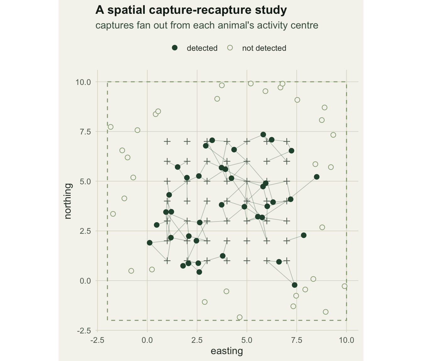

Figure 1: Trap grid (crosses), true activity centres (filled where detected, hollow where not), the state-space boundary (dashed), and links from each detected centre to the traps where it was caught. The spatial spread of an animal’s captures carries the movement information SCR uses.

The detection surface below shows the estimated probability that an animal centred at each point is caught at all. Its total is the effective sampling area: the array reaches beyond its own footprint but fades within a few sigma, which is exactly the region a fixed buffer tries, and fails, to guess.

gdf <- data.frame(x = G[, 1], y = G[, 2], pdot = pdh)
p2 <- ggplot(gdf, aes(x, y, fill = pdot)) +
  geom_raster(interpolate = TRUE) +
  geom_point(data = as.data.frame(traps), aes(x, y), inherit.aes = FALSE,
             shape = 3, colour = ink, size = 1.6, stroke = 0.5) +
  scale_fill_gradient(low = paper, high = forest, name = "P(detected)") +
  coord_equal() +
  labs(x = "easting", y = "northing",
       title = "Effective sampling area",
       subtitle = paste0("a_eff = ", round(a_eff, 1), " over a state-space of ", A)) +
  theme_te()
p2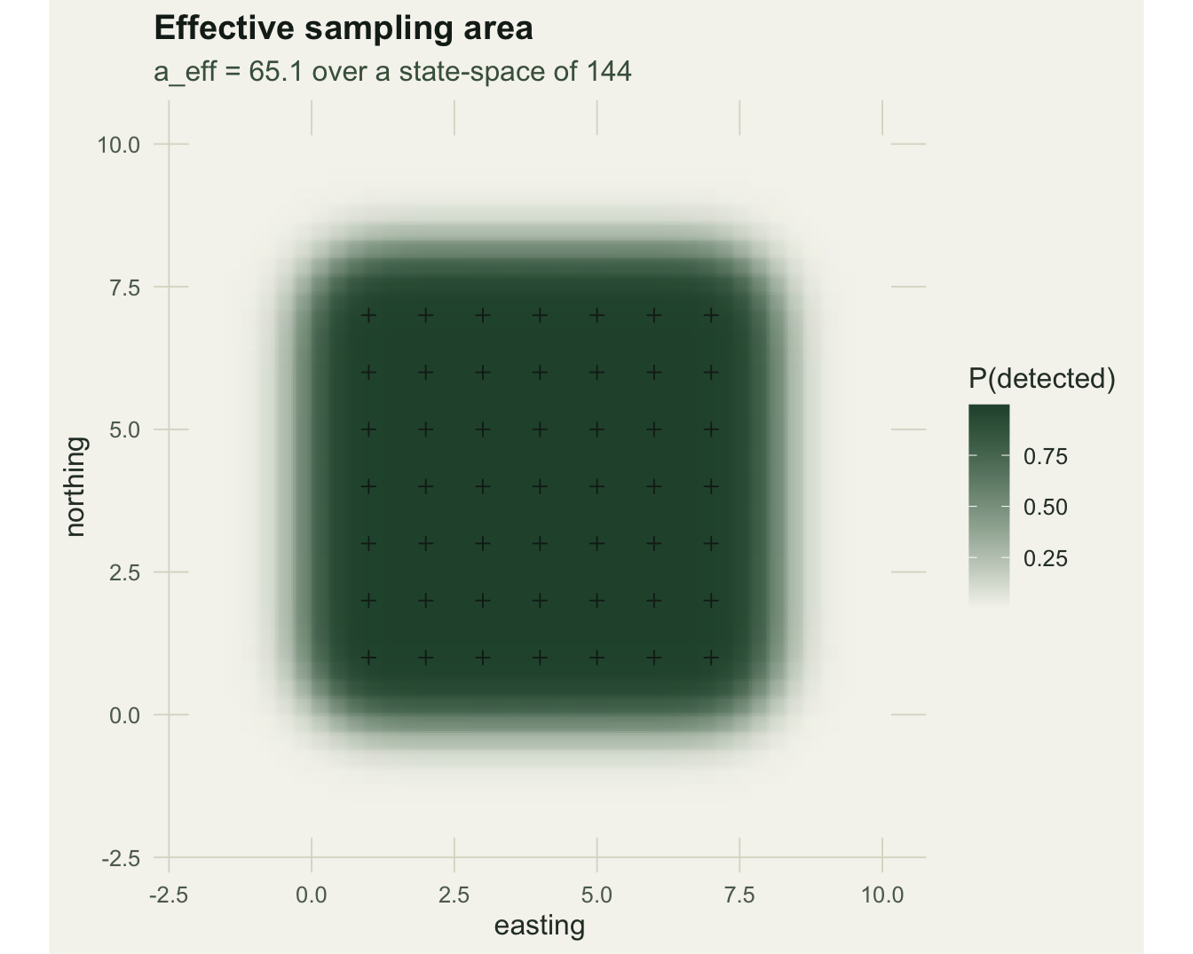

Figure 2: Estimated probability of detection as a function of an animal’s activity-centre location (paper to forest gradient), with traps overlaid. The integral of this surface is the effective sampling area; it extends past the array but decays smoothly, so no single buffer width reproduces it.

Takeaways

Non-spatial capture-recapture answers a question with no clean edge: how many animals were exposed to the array. Converting that to density needs an area that the data do not define, and the answer swings several-fold with the buffer you pick. SCR makes the activity centre a latent variable, ties detection to distance through g0 and sigma, and estimates density directly with a principled effective sampling area. The whole likelihood is a grid integral and an optim call; no specialised package is needed to see how it works. The spatial recaptures do the heavy lifting, so the next post looks at how trap spacing and array extent govern whether sigma, and therefore density, can be estimated with any precision.

References

Efford, M. 2004. Density estimation in live-trapping studies. Oikos 106(3):598-610 (10.1111/j.0030-1299.2004.13043.x).

Borchers, D. L. and Efford, M. G. 2008. Spatially explicit maximum likelihood methods for capture-recapture studies. Biometrics 64(2):377-385 (10.1111/j.1541-0420.2007.00927.x).

Efford, M. G., Borchers, D. L. and Byrom, A. E. 2009. Density estimation by spatially explicit capture-recapture: likelihood-based methods. In: Modeling Demographic Processes in Marked Populations, Springer (10.1007/978-0-387-78151-8_11).

Royle, J. A. and Young, K. V. 2008. A hierarchical model for spatial capture-recapture data. Ecology 89(8):2281-2289 (10.1890/07-0601.1).

Otis, D. L., Burnham, K. P., White, G. C. and Anderson, D. R. 1978. Statistical inference from capture data on closed animal populations. Wildlife Monographs 62:3-135 (10.2307/3830650).

Royle, J. A., Chandler, R. B., Sollmann, R. and Gardner, B. 2014. Spatial Capture-Recapture. Academic Press (ISBN 978-0-12-405939-9).

Related tutorials

• Closed-population capture-recapture
• Distance sampling for line transects
• Bayesian spatial capture-recapture
• N-mixture models for abundance