SCR sampling design and precision

How trap spacing relative to sigma controls spatial recaptures and the precision of density in spatial capture-recapture, worked from scratch in base R.

Spatial capture-recapture estimates density directly, but the precision of that estimate is not fixed: it is bought by the design. The single most important knob is the trap spacing relative to sigma, the spatial scale of detection. Space the traps too tightly and a small array catches few animals; space them too widely and almost no animal is caught at more than one trap, so sigma (and therefore density) drifts. Somewhere in between lies a spacing that estimates density with the least uncertainty for a fixed number of traps.

This post fixes the truth, sweeps the trap spacing across a range, and refits the from-scratch SCR likelihood many times at each spacing to measure the sampling variability of the density estimate. The result is a clear optimum, and a clear mechanism behind it.

Spatial recaptures are the currency

The frequentist post showed that sigma is pinned down by spatial recaptures: animals caught at two or more traps. A capture at a single trap says an animal was nearby, but not how far it typically ranges. The number of spatial recaptures depends on the geometry. With a fixed budget of traps, tight spacing covers a small area (few animals enter it) while each caught animal hits many traps (many recaptures); wide spacing covers a large area (many animals) but each animal usually touches one trap (few recaptures). Density precision has to trade these off.

One fit, then a sweep

The fitting function simulates a study at a given spacing (a 5 by 5 trap grid, a buffered state-space, activity centres from a Poisson process) and maximises the same integrated likelihood used in the basics post. It returns the density and sigma estimates plus the spatial-recapture count.

D_true <- 0.5; g0_true <- 0.30; sig_true <- 0.70; K <- 6

fit_one <- function(spacing) {
  tr    <- seq(0, 4 * spacing, by = spacing)          # 5 x 5 = 25 traps
  traps <- as.matrix(expand.grid(x = tr, y = tr)); J <- nrow(traps)
  buf   <- 4 * sig_true
  xl <- range(traps[, 1]) + c(-buf, buf); yl <- range(traps[, 2]) + c(-buf, buf)
  A  <- diff(xl) * diff(yl)
  N  <- rpois(1, D_true * A)
  sx <- runif(N, xl[1], xl[2]); sy <- runif(N, yl[1], yl[2])
  d2 <- outer(sx, traps[, 1], "-")^2 + outer(sy, traps[, 2], "-")^2
  Yf <- matrix(rbinom(N * J, K, g0_true * exp(-d2 / (2 * sig_true^2))), N, J)
  cc <- rowSums(Yf) > 0; Y <- Yf[cc, , drop = FALSE]; n <- nrow(Y)
  sr <- sum(rowSums(Y > 0) >= 2)
  if (n < 3) return(list(D = NA, sigma = NA, sr = sr, n = n, ok = FALSE))

  gx <- seq(xl[1], xl[2], length.out = 26); gy <- seq(yl[1], yl[2], length.out = 26)
  G  <- as.matrix(expand.grid(x = gx, y = gy))
  d2G <- outer(G[, 1], traps[, 1], "-")^2 + outer(G[, 2], traps[, 2], "-")^2
  Cc  <- rowSums(lchoose(K, Y))
  negll <- function(th) {                             # same likelihood as the basics post
    Dd <- exp(th[1]); g0 <- plogis(th[2]); sg <- exp(th[3])
    P  <- g0 * exp(-d2G / (2 * sg^2))
    pb <- mean(1 - exp(rowSums(K * log1p(-P))))
    if (pb <= 0) return(1e10)
    LM <- Y %*% t(log(P)) + (K - Y) %*% t(log1p(-P)) + Cc
    m  <- apply(LM, 1, max); lf <- m + log(rowMeans(exp(LM - m)))
    -(dpois(n, Dd * A * pb, log = TRUE) + sum(lf) - n * log(pb))
  }
  st <- c(log(max(n, 1) / (A * 0.4)), qlogis(0.25), log(sig_true))
  ft <- tryCatch(optim(st, negll, method = "BFGS",
                       control = list(maxit = 400, reltol = 1e-9)), error = function(e) NULL)
  if (is.null(ft) || ft$convergence != 0) return(list(D = NA, sigma = NA, sr = sr, n = n, ok = FALSE))
  Dh <- exp(ft$par[1]); sh <- exp(ft$par[3])
  list(D = Dh, sigma = sh, sr = sr, n = n,
       ok = is.finite(Dh) && is.finite(sh) && sh < 4 * sig_true && Dh < 5 * D_true)
}

Now sweep the spacing from well under sigma to several times sigma, with many replicate studies at each, and summarise the coefficient of variation of the density estimate.

set.seed(129)
spacings <- c(0.5, 0.75, 1.0, 1.5, 2.0, 2.5)
R <- 80
res <- data.frame()
for (sp in spacings) {
  Ds <- Ss <- SRs <- Ns <- oks <- numeric(R)
  for (r in 1:R) { o <- fit_one(sp); Ds[r] <- o$D; Ss[r] <- o$sigma
    SRs[r] <- o$sr; Ns[r] <- o$n; oks[r] <- o$ok }
  use <- oks == 1
  res <- rbind(res, data.frame(
    spacing = sp, sigma_ratio = sp / sig_true,
    n_mean = mean(Ns), sr_frac = mean(SRs / pmax(Ns, 1)), usable = mean(use),
    D_cv = sd(Ds[use]) / mean(Ds[use]), sig_cv = sd(Ss[use]) / mean(Ss[use])))
}
best <- res$spacing[which.min(res$D_cv)]

The precision curve is U-shaped. At the tightest spacing (0.71 sigma) the array is small and only about 11 animals are caught, so the density estimate has a coefficient of variation of 0.5: high, despite a healthy spatial-recapture fraction of 0.74. At the widest spacing (3.57 sigma) about 47 animals are caught, but the spatial-recapture fraction has collapsed to 0.06, sigma becomes hard to identify (some fits fail, giving a usable fraction of 0.98), and the density coefficient of variation climbs back to 0.22. The minimum sits at a spacing of 1.5 units, or 2.14 sigma, with a coefficient of variation of 0.17. That matches the standard guidance that traps should sit no more than about two sigma apart (Sun, Fuller and Royle 2014).

cvl <- pivot_longer(res, c(D_cv, sig_cv), names_to = "which", values_to = "cv")
cvl$which <- factor(cvl$which, c("D_cv", "sig_cv"), c("density CV", "sigma CV"))
bmin <- res[which.min(res$D_cv), ]
p1 <- ggplot(cvl, aes(sigma_ratio, cv, colour = which)) +
  geom_line(linewidth = 0.9) + geom_point(size = 1.8) +
  geom_point(data = bmin, aes(sigma_ratio, D_cv), colour = ink, size = 3.2, inherit.aes = FALSE) +
  annotate("text", x = bmin$sigma_ratio, y = bmin$D_cv, label = "optimum near 2 sigma",
           vjust = 2.2, hjust = 0.2, colour = ink, size = 3.3) +
  scale_colour_manual(values = c("density CV" = forest, "sigma CV" = rust), name = NULL) +
  labs(x = "trap spacing (units of sigma)", y = "coefficient of variation",
       title = "Density precision is U-shaped in trap spacing",
       subtitle = "too tight catches few animals; too wide loses spatial recaptures") +
  theme_te() + theme(legend.position = "top")
p1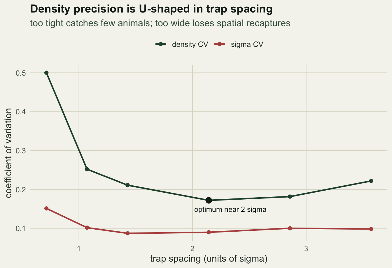

Figure 1: Coefficient of variation of the density estimate (and of sigma) against trap spacing in units of sigma, over many replicate studies at fixed trap number. Precision is worst at both extremes and best near two sigma, marked by the point.

The two forces behind the U

Splitting the drivers makes the trade-off explicit. As spacing widens, the number of animals detected rises steadily (more ground covered), while the fraction of animals recaptured at a second trap falls just as steadily (traps too far apart to both catch the same animal). Density precision needs both: enough animals for a stable count, and enough spatial recaptures to fix the detection scale. The optimum is where the two curves cross usefully, not where either is maximised.

dl <- pivot_longer(res, c(n_mean, sr_frac), names_to = "metric", values_to = "value")
dl$metric <- factor(dl$metric, c("n_mean", "sr_frac"),
                    c("animals detected", "spatial-recapture fraction"))
p2 <- ggplot(dl, aes(sigma_ratio, value)) +
  geom_line(colour = forest, linewidth = 0.9) + geom_point(colour = forest, size = 1.8) +
  facet_wrap(~ metric, scales = "free_y") +
  labs(x = "trap spacing (units of sigma)", y = NULL,
       title = "Coverage rises, recaptures fall",
       subtitle = "the density optimum needs a workable amount of both") +
  theme_te()
p2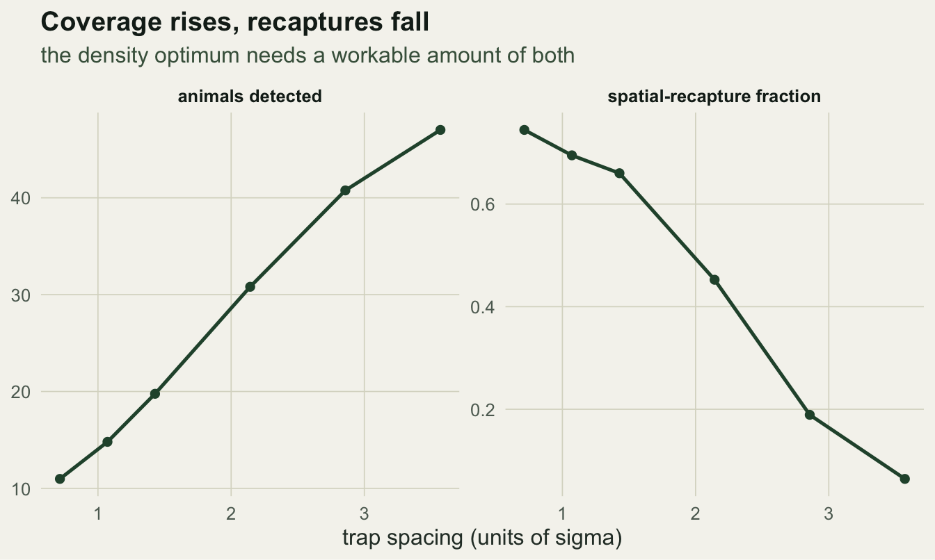

Figure 2: The two competing quantities against trap spacing: animals detected (rising with area) and the spatial-recapture fraction (falling as traps spread apart). The density optimum needs a workable amount of both, so it falls between the extremes rather than at either end.

Takeaways

The precision of an SCR density estimate is a design choice, not a given. Trap spacing relative to sigma sets it: too tight and the array is too small to catch many animals, too wide and the spatial recaptures that identify sigma disappear, with density uncertainty rising at both ends. For a fixed number of traps the sweet spot here is near two sigma, in line with the published recommendation. The practical implication is that you cannot plan an SCR study without a working guess at sigma (from a pilot, similar species, or telemetry), because the whole design hinges on it. The next post keeps the design fixed and turns to the detection process itself: covariates on g0, and how to check whether the fitted detection model actually fits.

References

Sun, C. C., Fuller, A. K. and Royle, J. A. 2014. Trap configuration and spacing influences parameter estimates in spatial capture-recapture models. PLoS ONE 9(2):e88025 (10.1371/journal.pone.0088025).

Efford, M. 2004. Density estimation in live-trapping studies. Oikos 106(3):598-610 (10.1111/j.0030-1299.2004.13043.x).

Borchers, D. L. and Efford, M. G. 2008. Spatially explicit maximum likelihood methods for capture-recapture studies. Biometrics 64(2):377-385 (10.1111/j.1541-0420.2007.00927.x).

Wilton, C. M., Puckett, E. E., Beringer, J., Gardner, B., Eggert, L. S. and Belant, J. L. 2014. Trap array configuration influences estimates and precision of black bear density and abundance. PLoS ONE 9(10):e111257 (10.1371/journal.pone.0111257).

Royle, J. A., Chandler, R. B., Sollmann, R. and Gardner, B. 2014. Spatial Capture-Recapture. Academic Press (ISBN 978-0-12-405939-9).

Related tutorials

• Spatial capture-recapture from scratch
• Detection covariates and checking in SCR
• Survey design for detection and visits
• Power analysis by simulation