---
title: "RDA vs CCA for community ecology: choosing by gradient length"
description: "When to use redundancy analysis versus canonical correspondence analysis on community data, why the DCA gradient-length rule decides it, and where the Hellinger transformation fits in."
date: "2026-06-23 10:00"
categories: [R, Ordination, Constrained ordination, Community ecology, vegan]
image: thumbnail.png
image-alt: "Two ordination panels: on a long gradient PCA scores bend back at the ends while CA scores stay ordered."
---
Redundancy analysis (RDA) and canonical correspondence analysis (CCA) are the two workhorses of constrained ordination, and a recurring question is which one to reach for. They are not interchangeable: they assume different things about how species respond to gradients, and the wrong choice can distort the picture or hide structure. The good news is that the decision has a simple, defensible answer, and it does not depend on taste. It depends on how long your gradient is.
## Two response models, two methods
RDA is constrained principal component analysis. It assumes species respond to a gradient in a roughly **linear** (monotonic) way over the sampled range, and it measures site dissimilarity with Euclidean distance. CCA is constrained correspondence analysis. It assumes species have **unimodal** responses, each with an optimum somewhere along the gradient, and it works in chi-square space (ter Braak 1986).
Real species responses are almost always unimodal: abundance rises to an optimum and falls away. So why is RDA ever appropriate? Because a short stretch of a bell curve looks like a straight line. If your sampled gradient covers only part of each species' range, the responses inside that window are effectively monotonic, and the linear model is fine. The longer the gradient, the more of the full bell each species shows, and the worse the linear approximation gets (ter Braak and Prentice 1988).
That is the whole tension. The practical job is to measure how long the gradient is.
## Two datasets: a short and a long gradient
We simulate communities from the honest generative model: each species has a Gaussian niche along one latent gradient. The only thing that changes between the two datasets is the **range** of gradient the sites span, relative to the niche widths. A narrow range gives mild turnover (a short gradient); a wide range gives strong turnover with many absences (a long gradient).
```{r}
#| label: setup
#| message: false
#| warning: false
library(vegan)
library(ggplot2)

pal_lo <- "#c9b458"; pal_hi <- "#1d5b4e"; ink <- "#16241d"; gline <- "#dad9ca"
th <- theme_minimal(base_size = 12) +
  theme(panel.grid.minor = element_blank(),
        panel.grid.major = element_line(color = gline, linewidth = 0.3),
        plot.title = element_text(face = "bold", size = 11.5, color = ink),
        legend.position = "right")

make_comm <- function(n, nsp, grad_range, tol, peak, seed, env_noise = 0.05) {
  set.seed(seed)
  g  <- runif(n, 0, grad_range)                         # site positions on the gradient
  u  <- seq(-0.4, grad_range + 0.4, length.out = nsp)   # species optima tile the range
  lam <- outer(g, u, function(gi, uj) peak * exp(-((gi - uj)^2) / (2 * tol^2)))
  comm <- matrix(rpois(length(lam), lam), nrow = n)     # Poisson counts around the niche
  colnames(comm) <- paste0("sp", seq_len(nsp))
  rownames(comm) <- paste0("s", seq_len(n))
  moisture <- as.numeric(scale(g)) + rnorm(n, 0, env_noise)  # measured proxy of the gradient
  ph <- rnorm(n)                                            # an independent null variable
  list(comm = comm, g = g, u = u, tol = tol, peak = peak,
       range = grad_range, moisture = moisture, ph = ph)
}

short <- make_comm(n = 45, nsp = 30, grad_range = 2.8, tol = 1.3, peak = 30, seed = 101)
long  <- make_comm(n = 45, nsp = 30, grad_range = 5.5, tol = 0.85, peak = 30, seed = 202)

c(short_zeros = mean(short$comm == 0), long_zeros = mean(long$comm == 0))
```
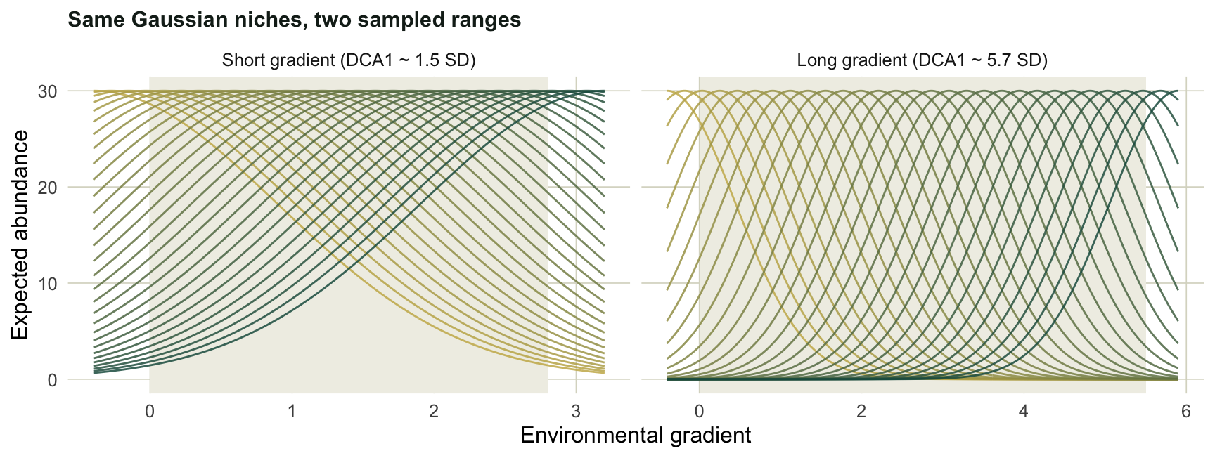
The short gradient has no empty cells; the long one is roughly a third zeros, because species drop out as you move away from their optimum. Plotting the niches makes the difference concrete. The shaded band marks the sampled sites.
```{r}
#| label: fig-responses
#| fig-width: 9
#| fig-height: 3.4
#| fig-cap: "The same Gaussian niches sampled over a narrow window (left, responses look monotonic) and a wide window (right, full bells and turnover)."
curve_df <- function(d, label) {
  xs <- seq(min(d$u), max(d$u), length.out = 400)
  do.call(rbind, lapply(seq_along(d$u), function(j)
    data.frame(x = xs, y = d$peak * exp(-((xs - d$u[j])^2) / (2 * d$tol^2)),
               sp = j, panel = label)))
}
lev <- c("Short gradient (DCA1 ~ 1.5 SD)", "Long gradient (DCA1 ~ 5.7 SD)")
cd  <- rbind(curve_df(short, lev[1]), curve_df(long, lev[2]))
cd$panel <- factor(cd$panel, levels = lev)
shade <- data.frame(panel = factor(lev, levels = lev), x1 = c(0, 0), x2 = c(2.8, 5.5))

ggplot(cd, aes(x, y, group = sp)) +
  geom_rect(data = shade, inherit.aes = FALSE,
            aes(xmin = x1, xmax = x2, ymin = -Inf, ymax = Inf), fill = "#f0efe6") +
  geom_line(aes(color = sp), linewidth = 0.5, alpha = 0.85) +
  scale_color_gradient(low = pal_lo, high = pal_hi, guide = "none") +
  facet_wrap(~panel, scales = "free_x") +
  labs(x = "Environmental gradient", y = "Expected abundance",
       title = "Same Gaussian niches, two sampled ranges") + th
```
## The decision tool: DCA gradient length
The standard way to measure gradient length is detrended correspondence analysis. Run it, then read the length of the first axis in standard-deviation units of species turnover. One SD unit is roughly the distance over which the community composition turns over by about half; a length of four means a near-complete turnover end to end (Hill and Gauch 1980). The rule of thumb is the one most ordination texts give: under about 3 SD, species behave monotonically and linear methods (RDA, PCA) are safe; over about 4 SD, the unimodal methods (CCA, CA) fit better; between 3 and 4, either is defensible.
```{r}
#| label: dca
#| message: false
#| warning: false
dca1 <- function(comm) {
  d <- decorana(comm)
  diff(range(scores(d, display = "sites", choices = 1)))  # axis-1 length in SD units
}
c(short = dca1(short$comm[, colSums(short$comm) > 0]),
  long  = dca1(long$comm[,  colSums(long$comm)  > 0]))
```
The short dataset comes out near 1.5 SD, well inside linear territory; the long one near 5.7 SD, firmly in unimodal territory. Note that we only use DCA to read the axis length. Its detrended axes themselves are best left uninterpreted, since the detrending rescales segments of the gradient in ways that can shuffle fine structure.
## What a long gradient does to a linear ordination
To see why the rule matters, drop the constraints for a moment and look at the plain unconstrained ordinations: PCA (the linear, Euclidean engine behind RDA) and CA (the unimodal, chi-square engine behind CCA). For each, take the first axis and ask how well it recovers the true gradient order.
```{r}
#| label: fig-recovery
#| fig-width: 9
#| fig-height: 3.6
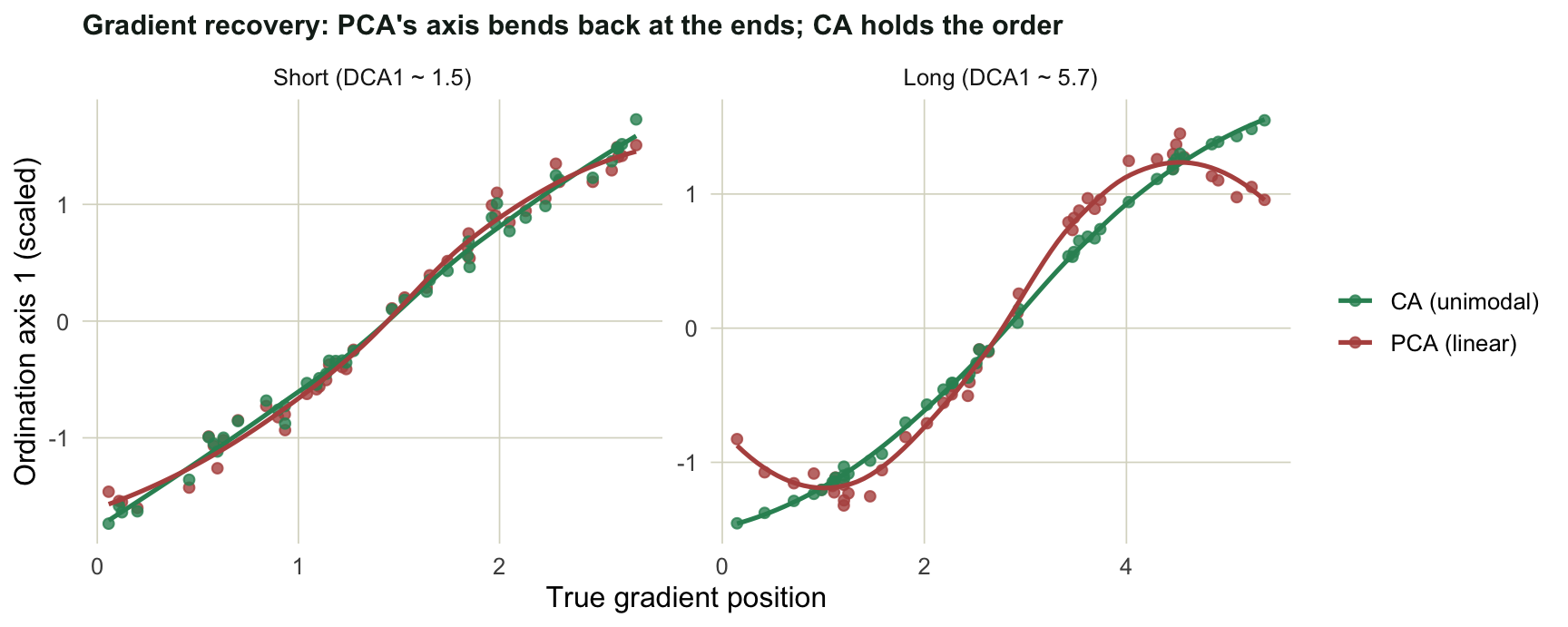
#| fig-cap: "First-axis scores against the true gradient. On the long gradient PCA's axis bends back at both ends (the horseshoe), while CA stays monotone."
rec <- function(d, label) {
  comm <- d$comm[, colSums(d$comm) > 0]
  p <- scores(rda(comm), display = "sites", choices = 1, scaling = 1)
  c <- scores(cca(comm), display = "sites", choices = 1, scaling = 1)
  if (cor(p, d$g) < 0) p <- -p
  if (cor(c, d$g) < 0) c <- -c
  rbind(data.frame(g = d$g, axis1 = as.numeric(scale(p)), method = "PCA (linear)",   grad = label),
        data.frame(g = d$g, axis1 = as.numeric(scale(c)), method = "CA (unimodal)", grad = label))
}
lev2 <- c("Short (DCA1 ~ 1.5)", "Long (DCA1 ~ 5.7)")
d2 <- rbind(rec(short, lev2[1]), rec(long, lev2[2]))
d2$grad <- factor(d2$grad, levels = lev2)

ggplot(d2, aes(g, axis1, color = method)) +
  geom_point(size = 1.7, alpha = 0.8) +
  geom_smooth(se = FALSE, method = "loess", formula = y ~ x, linewidth = 0.9) +
  scale_color_manual(values = c("PCA (linear)" = "#b5534e", "CA (unimodal)" = "#2f8f63"),
                     name = NULL) +
  facet_wrap(~grad, scales = "free") +
  labs(x = "True gradient position", y = "Ordination axis 1 (scaled)",
       title = "Gradient recovery: PCA's axis bends back at the ends; CA holds the order") + th
```
```{r}
#| label: recovery-numbers
recovery <- function(d) {
  comm <- d$comm[, colSums(d$comm) > 0]
  p <- scores(rda(comm), display = "sites", choices = 1, scaling = 1)
  c <- scores(cca(comm), display = "sites", choices = 1, scaling = 1)
  c(PCA = abs(cor(p, d$g, method = "spearman")),
    CA  = abs(cor(c, d$g, method = "spearman")))
}
rbind(short = recovery(short), long = recovery(long))
```
On the short gradient both axes track the gradient almost perfectly (rank correlation near 0.99 either way). On the long gradient CA still sits near 1.0, but PCA slips to around 0.92, and the figure shows why: the sites at the two extremes get pulled back toward the middle. This is the **double-zero problem**. Two sites at opposite ends of a long gradient share many species that are absent from both, and Euclidean distance reads those shared absences as similarity, so it folds the ends together into the classic horseshoe. Chi-square distance does not count joint absences the same way, so CA keeps the order.
The same long gradient also produces an arch, and it is easy to over-read. Plot the first two CA axes:
```{r}
#| label: fig-arch
#| fig-width: 6.4
#| fig-height: 4
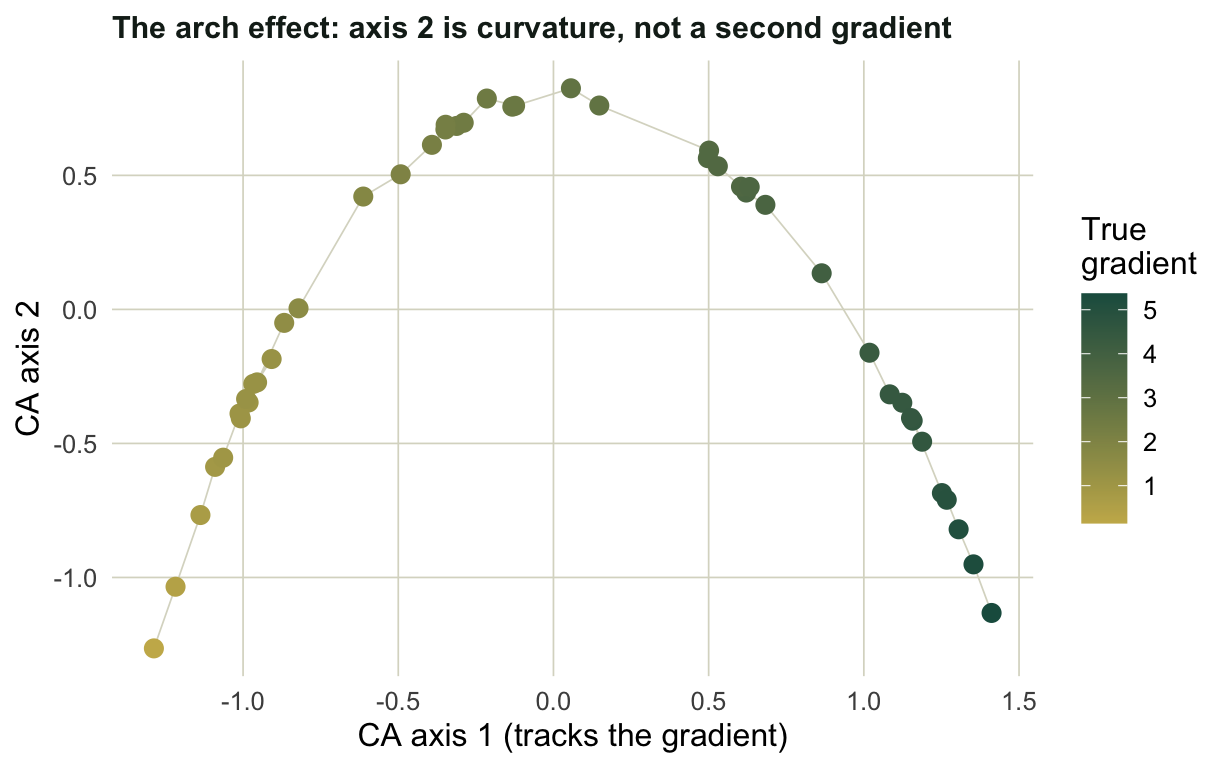
#| fig-cap: "On a single long gradient, axis 2 is a curved restatement of axis 1, not a second gradient."
commL <- long$comm[, colSums(long$comm) > 0]
sa <- scores(cca(commL), display = "sites", choices = 1:2, scaling = 1)
da <- data.frame(ax1 = sa[, 1], ax2 = sa[, 2], g = long$g)

ggplot(da, aes(ax1, ax2, color = g)) +
  geom_path(data = da[order(da$g), ], color = gline, linewidth = 0.3) +
  geom_point(size = 2.8) +
  scale_color_gradient(low = pal_lo, high = pal_hi, name = "True\ngradient") +
  labs(x = "CA axis 1 (tracks the gradient)", y = "CA axis 2",
       title = "The arch effect: axis 2 is curvature, not a second gradient") + th
```
The color runs cleanly from one end of axis 1 to the other, so axis 1 is the gradient. Axis 2 is just the parabola that a single strong gradient forces into the second dimension. Reading it as an independent ecological axis is one of the most common mistakes in ordination plots, and it is exactly what detrending was invented to suppress (Hill and Gauch 1980).
## Constraining on the driver: RDA against CCA
Now put the constraints back and run both methods properly, regressing the community on the measured driver (`moisture`) plus an independent null variable (`pH`) to keep the test honest, as in the [envfit and PERMANOVA post](../envfit-and-permanova/).
```{r}
#| label: constrained
#| message: false
#| warning: false
fit_both <- function(d, tag) {
  comm <- d$comm[, colSums(d$comm) > 0]
  env  <- data.frame(moisture = d$moisture, ph = d$ph)
  r <- rda(comm ~ moisture + ph, data = env)
  c <- cca(comm ~ moisture + ph, data = env)
  set.seed(1); ar <- anova(r, by = "terms", permutations = 999)
  set.seed(1); ac <- anova(c, by = "terms", permutations = 999)
  s1 <- scores(r, display = "sites", choices = 1)
  s2 <- scores(c, display = "sites", choices = 1)
  data.frame(
    method          = c("RDA", "CCA"),
    constrained_pct = round(100 * c(r$CCA$tot.chi / r$tot.chi, c$CCA$tot.chi / c$tot.chi), 1),
    adj_R2          = round(c(RsquareAdj(r)$adj.r.squared, RsquareAdj(c)$adj.r.squared), 2),
    moisture_F      = round(c(ar$F[1], ac$F[1]), 1),
    moisture_p      = c(ar$`Pr(>F)`[1], ac$`Pr(>F)`[1]),
    ph_p            = c(ar$`Pr(>F)`[2], ac$`Pr(>F)`[2]))
}
fit_both(short, "short")
fit_both(long, "long")
```
```{r}
#| label: agreement
#| message: false
#| warning: false
axis_cor <- function(d) {
  comm <- d$comm[, colSums(d$comm) > 0]
  env  <- data.frame(moisture = d$moisture, ph = d$ph)
  r <- scores(rda(comm ~ moisture + ph, env), display = "sites", choices = 1)
  c <- scores(cca(comm ~ moisture + ph, env), display = "sites", choices = 1)
  abs(cor(r, c))
}
c(short = axis_cor(short), long = axis_cor(long))
```
Here is the part that surprises people. Once you constrain on the variable that actually drives the community, RDA and CCA agree closely: their first constrained axes correlate near 0.98 even on the long gradient, both find `moisture` strongly significant, and both correctly leave the null `pH` non-significant. The gradient-length problem bites hardest in **exploratory** ordination, where you are letting the data show their own structure, and in how faithfully species and sites are placed. It bites much less in the significance test of a constraint you already named. So the choice between RDA and CCA is less about whether `moisture` "comes out significant" and more about which response model you trust the picture to be drawn under.
## The modern shortcut: transformation-based RDA
There is a third option that often makes the binary choice moot. The double-zero problem is a property of Euclidean distance, not of RDA itself. Apply a Hellinger transformation to the community data first, then run ordinary RDA on the transformed table. This **tb-RDA** keeps the whole linear, easily-extended RDA framework but gives it a distance that behaves well for community data with many zeros (Legendre and Gallagher 2001).
```{r}
#| label: tbrda
#| message: false
#| warning: false
commL <- long$comm[, colSums(long$comm) > 0]
H <- decostand(commL, "hellinger")
env <- data.frame(moisture = long$moisture, ph = long$ph)
tb  <- rda(H ~ moisture + ph, data = env)

h1 <- scores(rda(H), display = "sites", choices = 1, scaling = 1)
c(constrained_pct = round(100 * tb$CCA$tot.chi / tb$tot.chi, 1),
  recovery_spearman = round(abs(cor(h1, long$g, method = "spearman")), 3))
```
On the long gradient, tb-RDA recovers the gradient order at a rank correlation around 0.97, well above raw RDA's 0.92, even though CA still edges it. For most community data, tb-RDA is now the default many ecologists reach for first, with CCA reserved for genuinely long gradients where the unimodal model is the better description. The same Hellinger move underlies the [variance partitioning post](../variance-partitioning-varpart/).
## Where this leaves you
Run a DCA and read the first-axis length before you pick a constrained ordination. Under roughly 3 SD, the linear family is appropriate: use RDA, or tb-RDA on Hellinger-transformed data for a cleaner distance. Over roughly 4 SD, the unimodal family fits better: use CCA. In the 3 to 4 band either works, and tb-RDA is a reasonable hedge. Whatever you run, do not read axis 2 of a single-gradient ordination as a second gradient; check whether it is just the arch. And keep a null variable in the model so you know what non-significance looks like.
For the distance-based constrained ordination that handles arbitrary dissimilarities (including Bray-Curtis), see the [dbRDA post](../constrained-ordination-dbrda/) and the [capscale versus dbrda comparison](../capscale-vs-dbrda/); for the unconstrained side of the same data, the [NMDS post](../nmds-ordination/).
## References
ter Braak, C. J. F. (1986). Canonical correspondence analysis: a new eigenvector technique for multivariate direct gradient analysis. *Ecology* 67(5): 1167-1179. <https://doi.org/10.2307/1938672>
Hill, M. O. and Gauch, H. G. (1980). Detrended correspondence analysis: an improved ordination technique. *Vegetatio* 42: 47-58. <https://doi.org/10.1007/BF00048870>
ter Braak, C. J. F. and Prentice, I. C. (1988). A theory of gradient analysis. *Advances in Ecological Research* 18: 271-317. <https://doi.org/10.1016/S0065-2504(08)60183-X>
Legendre, P. and Gallagher, E. D. (2001). Ecologically meaningful transformations for ordination of species data. *Oecologia* 129: 271-280. <https://doi.org/10.1007/s004420100716>
Oksanen, J. et al. (2022). *vegan: Community Ecology Package*. R package version 2.6-4. <https://CRAN.R-project.org/package=vegan>