library(vegan)

set.seed(37)
S <- 24; n <- 60
x1 <- runif(n, -1, 1); x2 <- runif(n, -1, 1)
opt1 <- seq(-1.2, 1.2, length.out = S)
opt2 <- sample(seq(-1.2, 1.2, length.out = S))
lambda <- sapply(1:S, function(j)
  18 * exp(-0.5*((x1 - opt1[j])/0.6)^2 - 0.5*((x2 - opt2[j])/0.7)^2))
comm <- matrix(rpois(n * S, lambda), n, S)
comm[rowSums(comm) == 0, 1] <- 1
env <- data.frame(x1, x2)

D <- vegdist(comm, "bray")capscale vs dbrda: same axes, different test
R
ordination
vegan
multivariate
ecology tutorial
vegan has two functions for distance-based constrained ordination. On Bray-Curtis they return the same axes but a different pseudo-F: the negative eigenvalues.
The post on constrained ordination used dbrda to put environmental constraints on a Bray-Curtis dissimilarity. vegan has a second function for the same job, capscale, and most of the time the two are interchangeable. On a semimetric dissimilarity like Bray-Curtis they are not quite. They return the same constrained ordination, but a different pseudo-F, and the split happens at one specific place: the negative eigenvalues.
The two functions take different routes. capscale (Legendre and Anderson 1999) runs principal coordinates analysis on the dissimilarities, then ordinary RDA on the resulting coordinates. dbrda (McArdle and Anderson 2001) works directly on the double-centred distance matrix, without the intermediate coordinates. For a Euclidean distance the routes are equivalent. For a non-Euclidean one they diverge, because the dissimilarities cannot be embedded in real Euclidean space without an imaginary part, and that part shows up as negative eigenvalues.
A community and its dissimilarity
Two predictors drive composition; counts are Poisson around Gaussian niches. Bray-Curtis on this kind of data is semimetric, so it carries negative eigenvalues.
How non-Euclidean is this dissimilarity? Principal coordinates returns one eigenvalue per axis, and the negative ones are the imaginary part.
ev <- eigen(-0.5 * (diag(n) - 1/n) %*% as.matrix(D^2) %*% (diag(n) - 1/n),
            symmetric = TRUE, only.values = TRUE)$values
c(positive = sum(ev > 1e-8), negative = sum(ev < -1e-8),
  pct_negative = round(sum(abs(ev[ev < 0])) / sum(ev[ev > 0]) * 100, 1))
positive negative pct_negative
34.0 25.0 8.9 Many of the axes carry negative eigenvalues, and together they come to 8.9 per cent of the positive inertia. Small, but it is exactly what the two functions handle differently.
The same axes
cap <- capscale(D ~ x1 + x2, data = env, comm = comm)   # comm only feeds species scores
db  <- dbrda(D ~ x1 + x2, data = env)

cap
Call: capscale(formula = D ~ x1 + x2, data = env, comm = comm)

              Inertia Proportion Rank
Total         10.5194
RealTotal     11.5525     1.0000
Constrained    7.6692     0.6639    2
Unconstrained  3.8832     0.3361   34
Imaginary     -1.0330

Inertia is squared Bray distance

-- NOTE:
Species scores projected from 'comm'

Eigenvalues for constrained axes:
 CAP1  CAP2
4.489 3.180

Eigenvalues for unconstrained axes:
  MDS1   MDS2   MDS3   MDS4   MDS5   MDS6   MDS7   MDS8
0.8466 0.6682 0.2935 0.2225 0.1865 0.1839 0.1486 0.1219
(Showing 8 of 34 unconstrained eigenvalues)
db
Call: dbrda(formula = D ~ x1 + x2, data = env)

              Inertia Proportion Rank RealDims
Total         10.5194     1.0000
Constrained    7.6671     0.7288    2        2
Unconstrained  2.8523     0.2712   57       33

Inertia is squared Bray distance

Eigenvalues for constrained axes:
dbRDA1 dbRDA2
 4.488  3.179

Eigenvalues for unconstrained axes:
  MDS1   MDS2   MDS3   MDS4   MDS5   MDS6   MDS7   MDS8
0.8464 0.6680 0.2920 0.2224 0.1844 0.1770 0.1484 0.1201
(Showing 8 of 57 unconstrained eigenvalues)
Read the two partition tables together. Total inertia is the same. The constrained inertia is the same to three figures, a little over seventy per cent of the total in both. The constrained eigenvalues match to two decimal places: CAP1 4.489 against dbRDA1 4.488, CAP2 3.180 against dbRDA2 3.179. As a constrained ordination the two results are the same picture.
The difference is in the bookkeeping below the constrained part. capscale reports an Imaginary line: it has set the negative-eigenvalue inertia aside, outside both the constrained and the real unconstrained totals. dbrda has no imaginary line; its unconstrained total already nets the negative eigenvalues against the positive ones, which is why its unconstrained inertia is smaller.
rbind(
  capscale = c(adjR2 = RsquareAdj(cap)$adj.r.squared,
               resid = cap$CA$tot.chi),
  dbrda    = c(adjR2 = RsquareAdj(db)$adj.r.squared,
               resid = db$CA$tot.chi))
adjR2 resid
capscale 0.6520672 3.883228
dbrda 0.7193353 2.852350The adjusted R-squared values are not the same: 0.65 for capscale against 0.72 for dbrda. The constrained inertia behind them agrees to three figures; what differs is the total each function divides it by. capscale divides by the real total, which leaves the imaginary inertia outside and so is the larger denominator, while dbrda divides by a total that has already netted the negative eigenvalues away. The residual inertia splits for the same reason.
A different denominator, a different F
The permutation test divides constrained variation by residual variation. Same numerator, different residual, different pseudo-F.
set.seed(1); ac <- anova(cap, permutations = 999)
set.seed(1); ad <- anova(db,  permutations = 999)
c(capscale_F = round(ac$F[1], 1), dbrda_F = round(ad$F[1], 1),
  capscale_p = ac$`Pr(>F)`[1], dbrda_p = ad$`Pr(>F)`[1])
capscale_F dbrda_F capscale_p dbrda_p
56.300 76.600 0.001 0.001 The dbRDA pseudo-F comes out larger, near seventy-seven against fifty-six. The mechanism is direct: dbrda subtracts the negative-eigenvalue inertia from the residual, so its denominator is smaller, so its F is larger. Here both p values land at the permutation floor and the conclusion is the same, but in a borderline case the choice of function could move the p value across a threshold. When the test is the point, that matters.
This is the residual structure that drives the gap:
ca <- db$CA$eig
dfe <- data.frame(idx = seq_along(ca), eig = as.numeric(ca),
                  sign = ifelse(ca < 0, "negative", "positive"))
ggplot(dfe, aes(idx, eig, fill = sign)) +
  geom_col(width = .85) +
  geom_hline(yintercept = 0, color = pal$body, linewidth = .3) +
  scale_fill_manual(values = c(positive = pal$forest, negative = pal$terra), name = NULL) +
  labs(x = "Residual (unconstrained) axis", y = "Eigenvalue") + th()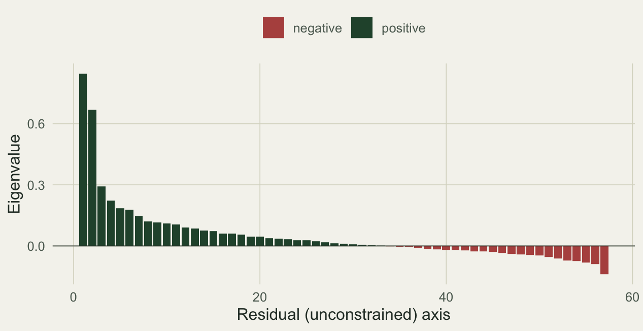
And the constrained ordination itself, which both functions agree on:
si <- as.data.frame(scores(db, display = "sites", choices = 1:2)); si$x1 <- x1
bp <- as.data.frame(scores(db, display = "bp", choices = 1:2))
mul <- 0.9 * max(abs(unlist(si[, 1:2]))) / max(sqrt(rowSums(bp^2)))
bp <- bp * mul
eig <- round(100 * db$CCA$eig / db$tot.chi, 1)

ggplot(si, aes(dbRDA1, dbRDA2, color = x1)) +
  geom_point(size = 2.4) +
  scale_color_gradient(low = pal$low, high = pal$high, name = "first predictor") +
  geom_segment(data = bp, aes(0, 0, xend = dbRDA1, yend = dbRDA2), inherit.aes = FALSE,
               arrow = arrow(length = unit(.18, "cm")), color = pal$terra, linewidth = .6) +
  geom_text(data = bp, aes(dbRDA1, dbRDA2,
                           label = c(x1 = "first predictor", x2 = "second predictor")[rownames(bp)]),
            inherit.aes = FALSE, color = pal$terra, vjust = -.5, size = 3.5) +
  labs(x = paste0("dbRDA1 (", eig[1], "%)"), y = paste0("dbRDA2 (", eig[2], "%)")) + th()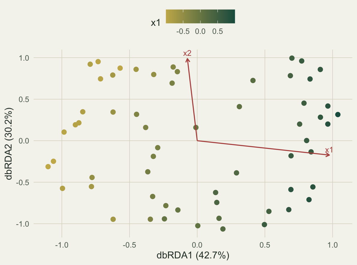
With a Euclidean distance they agree exactly
Hellinger distance is Euclidean, so it produces no negative eigenvalues and no imaginary part. With nothing to treat differently, the two functions return the same constrained inertia to numerical precision.
DH <- dist(decostand(comm, "hellinger"))
capH <- capscale(DH ~ x1 + x2, data = env)
dbH  <- dbrda(DH ~ x1 + x2, data = env)
c(capscale = capH$CCA$tot.chi, dbrda = dbH$CCA$tot.chi,
  difference = abs(capH$CCA$tot.chi - dbH$CCA$tot.chi))
capscale dbrda difference
1.518764e+01 1.518764e+01 1.598721e-14 The difference is at the rounding limit. The whole divergence on Bray-Curtis was the negative eigenvalues, and a Euclidean distance has none.
One practical difference, and what to use
capscale can give you species scores, which is convenient for a biplot, but not from a dissimilarity object alone. When the left-hand side of the formula is a dist, the species table has to be handed over separately as comm, which is why the fit above was called with comm = comm. dbrda has no such argument at all, for the reason covered in the dbRDA post: the analysis runs on the double-centred distance matrix, not on a species table, so species coordinates only appear if you add them afterwards with sppscores.
cap_bare <- capscale(D ~ x1 + x2, data = env)   # same fit, no species table handed over
grab <- function(m) tryCatch(scores(m, display = "species", choices = 1:2),
                             error = function(e) NULL)
count <- function(s) if (is.null(s) || all(is.na(s))) "none" else nrow(s)

list(capscale_without_comm = count(grab(cap_bare)),
     capscale_with_comm    = count(grab(cap)),
     dbrda_species_scores  = count(grab(db)))
$capscale_without_comm
[1] "none"
$capscale_with_comm
[1] 24
$dbrda_species_scores
[1] "none"The recommendation follows the mechanism. When the dissimilarity is metric or Euclidean (Hellinger, chord, Euclidean), the two functions agree, so use either; capscale with comm supplied is convenient if you want species scores for the biplot. When the dissimilarity is semimetric (Bray-Curtis, Jaccard) and the test is what you report, prefer dbrda: it partitions the variation directly from the distance matrix, including the non-Euclidean part, which is the partition McArdle and Anderson (2001) argued for. If you would rather stay with capscale on a semimetric dissimilarity, the negative eigenvalues can be removed first, by taking square roots of the dissimilarities or by adding a constant (add = TRUE); the vegan help documents both.
A note on the name. capscale takes its label from CAP, the canonical analysis of principal coordinates of Anderson and Willis (2003). That method is a discriminant or correlation analysis on principal coordinates, aimed at an a priori hypothesis, and it is not identical to what capscale computes, which is RDA on principal coordinates. The family is the same; the exact engine is not.
References
Legendre P, Anderson MJ 1999 Ecological Monographs 69(1):1-24 (10.1890/0012-9615(1999)069[0001:DBRATM]2.0.CO;2)
McArdle BH, Anderson MJ 2001 Ecology 82(1):290-297 (10.1890/0012-9658(2001)082[0290:FMMTCD]2.0.CO;2)
Anderson MJ, Willis TJ 2003 Ecology 84(2):511-525 (10.1890/0012-9658(2003)084[0511:CAOPCA]2.0.CO;2)
Oksanen J, Simpson GL, Blanchet FG, et al. 2022 vegan: Community Ecology Package, R package version 2.6-4 (https://CRAN.R-project.org/package=vegan)