Pseudo-absence and background points for SDMs

How many background points an SDM needs, why predicted values are relative rather than probabilities, and how case weights stabilise the scale, worked in R.

A presence-only dataset has no zeros. To fit a binomial GLM, a logistic regression, or most other correlative models, you need something to contrast the presences against: a sample of the conditions available across the region, labelled absent. These points go by two names. Pseudo-absences are treated as if they were surveyed absences, usually few and sometimes placed away from known presences. Background points simply describe the available environment, usually many and drawn at random. The distinction matters less than three decisions that both share: how many points, where they come from, and how they are weighted. This post works through all three on the same synthetic landscape used to build the baseline SDM.

library(terra)
library(dplyr)
library(ggplot2)
library(tidyr)

pal_paper <- "#f5f4ee"; pal_ink <- "#16241d"; pal_body <- "#2c3a31"
pal_forest <- "#275139"; pal_label <- "#46604a"; pal_line <- "#dad9ca"; pal_faint <- "#5d6b61"
pal_gold <- "#c9b458"; pal_red <- "#b5534e"
theme_te <- function(base_size = 12) {
  theme_minimal(base_size = base_size) +
    theme(text = element_text(colour = pal_body),
          plot.title = element_text(colour = pal_ink, face = "bold", size = rel(1.05)),
          plot.subtitle = element_text(colour = pal_faint),
          axis.title = element_text(colour = pal_label), axis.text = element_text(colour = pal_body),
          panel.grid.minor = element_blank(),
          panel.grid.major = element_line(colour = pal_line, linewidth = 0.3),
          strip.text = element_text(colour = pal_ink, face = "bold"),
          legend.title = element_text(colour = pal_label),
          plot.background = element_rect(fill = pal_paper, colour = NA),
          panel.background = element_rect(fill = "white", colour = NA),
          legend.key = element_rect(fill = pal_paper, colour = NA), legend.position = "top")
}

set.seed(42)
r_template <- rast(nrows = 80, ncols = 80, xmin = 0, xmax = 80, ymin = 0, ymax = 80)
xy <- xyFromCell(r_template, 1:ncell(r_template))
temp_trend <- 22 - 0.18 * xy[, "y"]
temp_noise <- rast(r_template); values(temp_noise) <- rnorm(ncell(r_template), 0, 2)
temp_noise <- focal(temp_noise, w = 9, fun = mean, na.rm = TRUE)
temp <- rast(r_template); values(temp) <- temp_trend; temp <- temp + temp_noise; names(temp) <- "temp"
prec_trend <- 500 + 5 * xy[, "x"]
prec_noise <- rast(r_template); values(prec_noise) <- rnorm(ncell(r_template), 0, 60)
prec_noise <- focal(prec_noise, w = 9, fun = mean, na.rm = TRUE)
prec <- rast(r_template); values(prec) <- prec_trend; prec <- prec + prec_noise; names(prec) <- "prec"
env <- c(temp, prec)
temp_v <- values(temp)[, 1]; prec_v <- values(prec)[, 1]

suit_true <- exp(-((temp_v - 15)^2) / (2 * 2.2^2)) * exp(-((prec_v - 800)^2) / (2 * 110^2))
set.seed(101)
pres_cells <- sample(ncell(r_template), 300, prob = suit_true, replace = FALSE)
pres_df <- data.frame(pa = 1, temp = temp_v[pres_cells], prec = prec_v[pres_cells])

The species has 300 occurrence records, its optimum sits at 15 degrees and 800 mm, and the true niche is known only because the landscape is simulated. Everything below is a decision about the zero class.

How many background points

Background points sample the available environment, so too few of them describe it poorly and the fitted niche wanders. To see how much, draw background sets of increasing size, fit the GLM each time, and record the estimated temperature optimum (the peak of the response curve). Repeating the draw 40 times at each size shows the spread, not just one lucky fit.

opt_from_fit <- function(m, dat) {
  ts <- seq(min(dat$temp), max(dat$temp), length.out = 200)
  ps <- seq(min(dat$prec), max(dat$prec), length.out = 200)
  c(temp_opt = ts[which.max(predict(m, data.frame(temp = ts, prec = median(dat$prec)), type = "response"))],
    prec_opt = ps[which.max(predict(m, data.frame(temp = median(dat$temp), prec = ps), type = "response"))])
}
n_grid <- c(50, 100, 250, 500, 1000, 2500, 5000)
set.seed(303)
res1 <- do.call(rbind, lapply(n_grid, function(nb) {
  t(sapply(1:40, function(i) {
    bgc <- sample(ncell(r_template), nb)
    d <- rbind(pres_df, data.frame(pa = 0, temp = temp_v[bgc], prec = prec_v[bgc]))
    d <- d[complete.cases(d), ]
    m <- glm(pa ~ poly(temp, 2) + poly(prec, 2), data = d, family = binomial)
    c(n_bg = nb, opt_from_fit(m, d))
  }))
}))
res1 <- as.data.frame(res1)
res1 %>% group_by(n_bg) %>%
  summarise(temp_sd = round(sd(temp_opt), 3), temp_mean = round(mean(temp_opt), 2),
            prec_sd = round(sd(prec_opt), 1), .groups = "drop")

# A tibble: 7 × 4
   n_bg temp_sd temp_mean prec_sd
  <dbl>   <dbl>     <dbl>   <dbl>
1    50   0.226      14.8    39.3
2   100   0.201      14.9    29.9
3   250   0.137      14.9    15  
4   500   0.099      14.9    12.4
5  1000   0.061      14.9     8.5
6  2500   0.038      14.9     4  
7  5000   0.034      14.9     1.7

The mean estimate sits near 14.9 at every size, so more background points do not move the answer, they sharpen it. The scatter in the estimated temperature optimum falls from a standard deviation of 0.23 at 50 points to 0.03 at 5000; for precipitation it falls from 39 to under 2. Below a few hundred points the niche estimate is visibly noisy.

res1_f <- res1 %>% mutate(n_bg = factor(n_bg, levels = n_grid))
ggplot(res1_f, aes(n_bg, temp_opt)) +
  geom_hline(yintercept = 15, colour = pal_red, linetype = "dashed") +
  geom_jitter(width = 0.12, height = 0, colour = pal_forest, alpha = 0.4, size = 1) +
  stat_summary(fun = mean, geom = "point", colour = pal_ink, size = 2.4) +
  annotate("text", x = 6.7, y = 15.5, label = "true optimum", colour = pal_red, hjust = 1, size = 3.3) +
  labs(title = "Estimated temperature optimum by number of background points",
       subtitle = "40 background draws per level; black points are the mean of each",
       x = "Number of background points", y = "Estimated optimum (C)") +
  theme_te(12) + theme(legend.position = "none")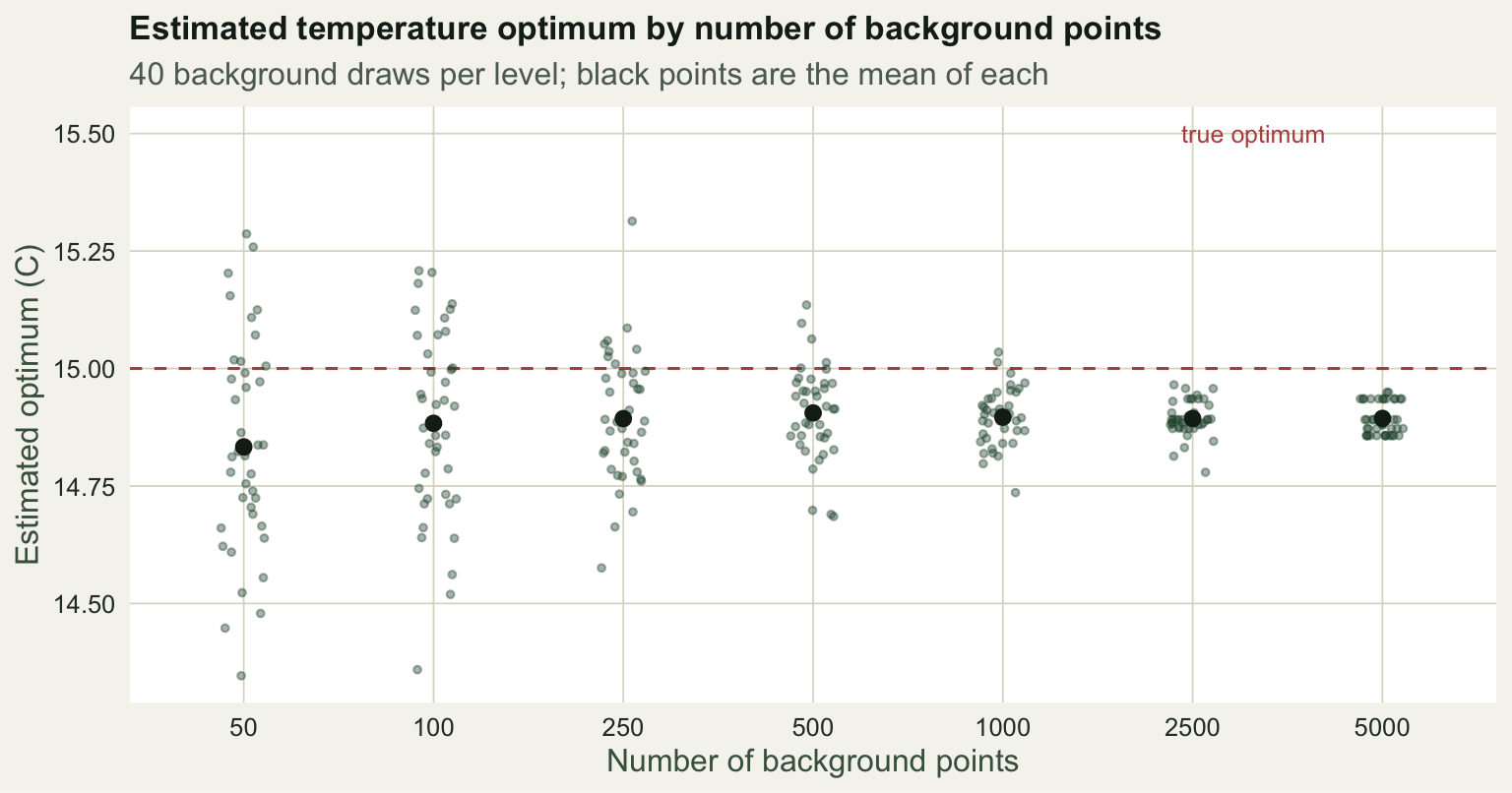

Figure 1: Estimated temperature optimum against background sample size. Each point is one of 40 draws; black points are the means.

A common default is a large random background, in the thousands, precisely so this sampling noise stops mattering. The cost is only computation.

Predicted values are relative, not probabilities

There is a catch that more points cannot fix. The ratio of presences to background is something you choose, and that ratio sets the intercept of the logistic model. Change the number of background points and the predicted values shift up or down, even though the fitted shape does not move. Fit the same model with 500 and with 5000 background points and compare.

fit_glm <- function(nb, seed, weighted = FALSE) {
  set.seed(seed); bgc <- sample(ncell(r_template), nb)
  d <- rbind(pres_df, data.frame(pa = 0, temp = temp_v[bgc], prec = prec_v[bgc]))
  d <- d[complete.cases(d), ]
  w <- if (weighted) ifelse(d$pa == 1, 1, sum(d$pa == 1) / sum(d$pa == 0)) else rep(1, nrow(d))
  glm(pa ~ poly(temp, 2) + poly(prec, 2), data = d, family = binomial, weights = w)
}
m_500 <- fit_glm(500, 11); m_5000 <- fit_glm(5000, 11)
axis_t <- seq(min(temp_v), max(temp_v), length.out = 200)
curve_t <- function(m) predict(m, data.frame(temp = axis_t, prec = median(pres_df$prec)), type = "response")
c(intercept_500 = round(coef(m_500)[[1]], 2), intercept_5000 = round(coef(m_5000)[[1]], 2),
  peak_500 = round(max(curve_t(m_500)), 2), peak_5000 = round(max(curve_t(m_5000)), 2))

 intercept_500 intercept_5000       peak_500      peak_5000 
         -0.93          -3.80           0.72           0.20 

The intercept drops from -0.93 to -3.80 and the peak of the response curve falls from 0.72 to 0.20. The optimum is unchanged at 14.9 in both. The two surfaces rank cells identically:

v500  <- values(terra::predict(env, m_500,  type = "response", na.rm = TRUE))[, 1]
v5000 <- values(terra::predict(env, m_5000, type = "response", na.rm = TRUE))[, 1]
round(cor(v500, v5000, method = "spearman", use = "complete.obs"), 3)

[1] 1

A Spearman correlation of 1.00 means the ranking of suitability across the landscape is the same; only the numbers on the scale differ. This is the single most misread property of a presence-background SDM: the output is a relative suitability index, not a probability of occurrence. Reporting a cell as “0.72 suitable” is meaningless without stating the background used to produce it.

The fix comes from point-process theory. Down-weighting the background so its total weight equals the number of presences makes logistic regression approximate the intensity of an inhomogeneous Poisson process, and the predicted scale stops depending on how many background points you drew.

mw_500 <- fit_glm(500, 11, weighted = TRUE); mw_5000 <- fit_glm(5000, 11, weighted = TRUE)
c(weighted_peak_500 = round(max(curve_t(mw_500)), 2),
  weighted_peak_5000 = round(max(curve_t(mw_5000)), 2))

 weighted_peak_500 weighted_peak_5000 
              0.81               0.81 

With weights the peak lands at 0.81 for both sample sizes. The figure puts the two schemes side by side: unweighted, the curves separate by sample size; weighted, they coincide.

resp2 <- rbind(
  data.frame(temp = axis_t, y = curve_t(m_500),   n_bg = "500",  scheme = "Unweighted"),
  data.frame(temp = axis_t, y = curve_t(m_5000),  n_bg = "5000", scheme = "Unweighted"),
  data.frame(temp = axis_t, y = curve_t(mw_500),  n_bg = "500",  scheme = "Down-weighted background"),
  data.frame(temp = axis_t, y = curve_t(mw_5000), n_bg = "5000", scheme = "Down-weighted background"))
resp2$scheme <- factor(resp2$scheme, levels = c("Unweighted", "Down-weighted background"))
ggplot(resp2, aes(temp, y, colour = n_bg)) +
  geom_line(linewidth = 1) +
  facet_wrap(~scheme) +
  scale_colour_manual(values = c("500" = pal_gold, "5000" = pal_forest), name = "Background points") +
  labs(title = "Predicted values are relative, not probabilities",
       subtitle = "Same presences and same niche shape; only the vertical scale moves",
       x = "Temperature (C)", y = "Predicted value") +
  theme_te(12)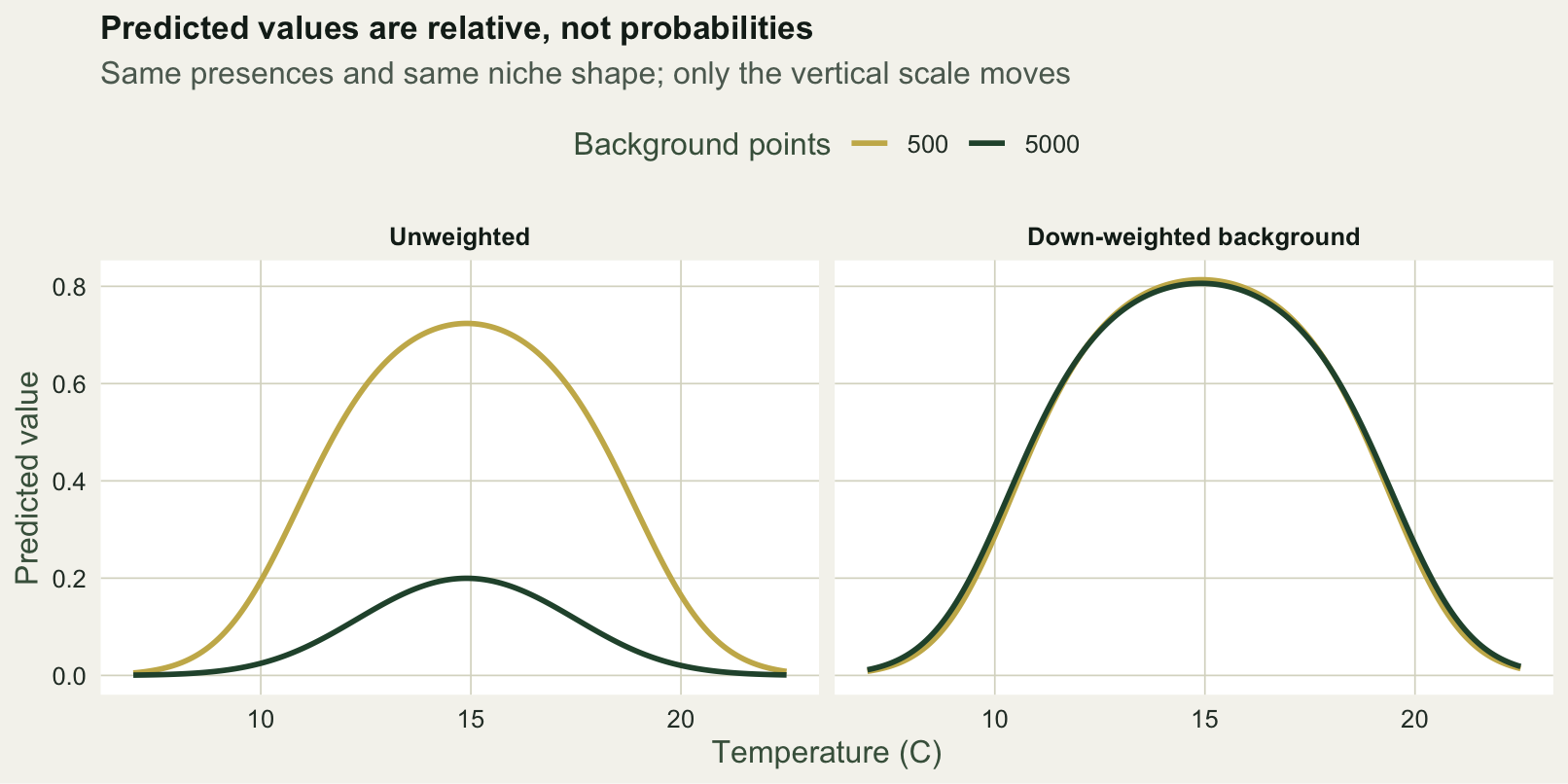

Figure 2: Temperature response under two background sizes, unweighted and with down-weighted background.

Where the background comes from

The third decision has no tidy figure here but often matters most. Background drawn uniformly at random describes the whole region, which is the right reference only if occurrences were collected evenly across it. They rarely are. Records cluster near roads, towns and reserves, so the presences carry a sampling bias that random background does not share, and the model then partly fits survey effort rather than the species. One remedy is to draw background with the same bias as the occurrences, for example a target-group background built from records of similar, similarly surveyed species (Phillips et al. 2009).

Restricting the background to an accessible area, a buffer around the occurrences or a dispersal-limited region, changes the question the model answers. A wide background asks which conditions the species prefers across everything on offer; a narrow one asks how it sorts within the range it could plausibly reach. Neither is wrong, but they give different response curves, and the choice should follow the ecology, not the default (Barbet-Massin et al. 2012).

Recommendations

Use a large random background, in the low thousands, unless you have a specific reason not to; this removes the sampling noise from the first section. Treat the predictions as a relative index, and if you need a stable or comparable scale across models, weight the background as above. State plainly how many background points you used and where they came from, because as this post shows, both are part of the model rather than incidental settings. The next step is measuring whether any of it predicts held-out occurrences, which is where evaluation comes in.

References

• Barbet-Massin M, Jiguet F, Albert CH, Thuiller W 2012. Methods in Ecology and Evolution 3(2):327-338 (10.1111/j.2041-210X.2011.00172.x)
• Phillips SJ, Dudik M, Elith J, Graham CH, Lehmann A, Leathwick J, Ferrier S 2009. Ecological Applications 19(1):181-197 (10.1890/07-2153.1)
• Warton DI, Shepherd LC 2010. The Annals of Applied Statistics 4(3):1383-1402 (10.1214/10-AOAS331)
• Guisan A, Zimmermann NE 2000. Ecological Modelling 135(2-3):147-186 (10.1016/S0304-3800(00)00354-9)

Related tutorials

• Species distribution modelling with GLM in R
• Logistic regression for presence-absence data
• Cleaning GBIF and iNaturalist records in R
• Evaluating species distribution models in R