---
title: "From GLM coefficients to predicted values in R"
description: "Turn count and logistic GLM coefficients into predicted values in R: build the confidence band on the link scale, back-transform it, and read the effect correctly."
date: "2026-06-26 10:00"
categories: [GLM, prediction, count data, logistic regression]
image: thumbnail.png
image-alt: "A fitted curve shown twice, as a straight line with an even band on the log scale and as a bending curve with a lopsided band on the count scale."
---
A negative binomial model of abundance hands you a table of coefficients on the log scale. The figure a reviewer actually wants is predicted abundance against the gradient, with a confidence band, on the count scale. Getting from one to the other has a single rule, and skipping it produces a band that is the wrong shape and can stray outside the values a count or a probability is allowed to take.
The coefficient lines we wrote earlier ([count GLMs](../glm-count-data-abundance/), [presence/absence](../logistic-regression-presence-absence/)) stopped at reading the numbers. This one turns those numbers into the predicted curve you publish.
## A model to predict from
We simulate overdispersed counts that rise with canopy openness and fall with elevation, then fit a negative binomial GLM. The covariate `elev_z` is standardised, so its mean is zero by construction.
```{r}
#| label: data
#| warning: false
#| message: false
library(MASS)
library(ggplot2)

set.seed(53)
n      <- 200
canopy <- runif(n, 0.05, 0.95)        # canopy openness, the focal predictor
elev_z <- rnorm(n)                    # standardised elevation, a covariate
mu     <- exp(1.0 + 2.2 * canopy - 0.5 * elev_z)
count  <- rnbinom(n, size = 2, mu = mu)
dat    <- data.frame(count, canopy, elev_z)

m <- glm.nb(count ~ canopy + elev_z, data = dat)
round(coef(m), 3)
```
```{r}
#| label: setup
#| include: false
ink<-"#16241d"; body<-"#2c3a31"; forest<-"#275139"; gold<-"#c9b458"
paper<-"#f5f4ee"; line<-"#dad9ca"; faint<-"#5d6b61"
theme_te <- function(){
theme_minimal(base_size = 12) +
theme(plot.background=element_rect(fill=paper,colour=NA),
panel.background=element_rect(fill=paper,colour=NA),
panel.grid.minor=element_blank(),
panel.grid.major=element_line(colour=line,linewidth=.3),
axis.title=element_text(colour=ink), axis.text=element_text(colour=faint),
plot.title=element_text(colour=ink,size=12,face="bold"),
strip.text=element_text(colour=ink,face="bold"),
legend.position="bottom", legend.title=element_text(colour=ink),
legend.text=element_text(colour=body))
}
crit <- qnorm(0.975)
```
The canopy coefficient is about 2.06. That is not a count and it is not a slope in individuals per unit; it lives on the log scale, where the model is linear. Exponentiating it gives 7.83 (95% CI 5.15 to 11.90), a multiplicative factor we will come back to. To get an actual predicted count we have to leave the log scale, and that step is where the band is usually mishandled.
## Build the interval on the link scale, then transform
`predict()` will return the fitted values and their standard errors on either scale. The rule is to ask for the **link** scale, form the interval there with a symmetric `fit +/- 1.96 * se`, and only then apply the inverse link (`exp` for a log link). The interval inherits the link's range, so a back-transformed count band can never go below zero.
```{r}
#| label: predict-grid
grid <- data.frame(canopy = seq(0.05, 0.95, length.out = 100), elev_z = 0)
pl   <- predict(m, newdata = grid, type = "link", se.fit = TRUE)

grid$mu <- exp(pl$fit)                          # predicted mean count
grid$lo <- exp(pl$fit - crit * pl$se.fit)       # lower 95% limit
grid$hi <- exp(pl$fit + crit * pl$se.fit)       # upper 95% limit
head(round(grid, 2), 3)
```
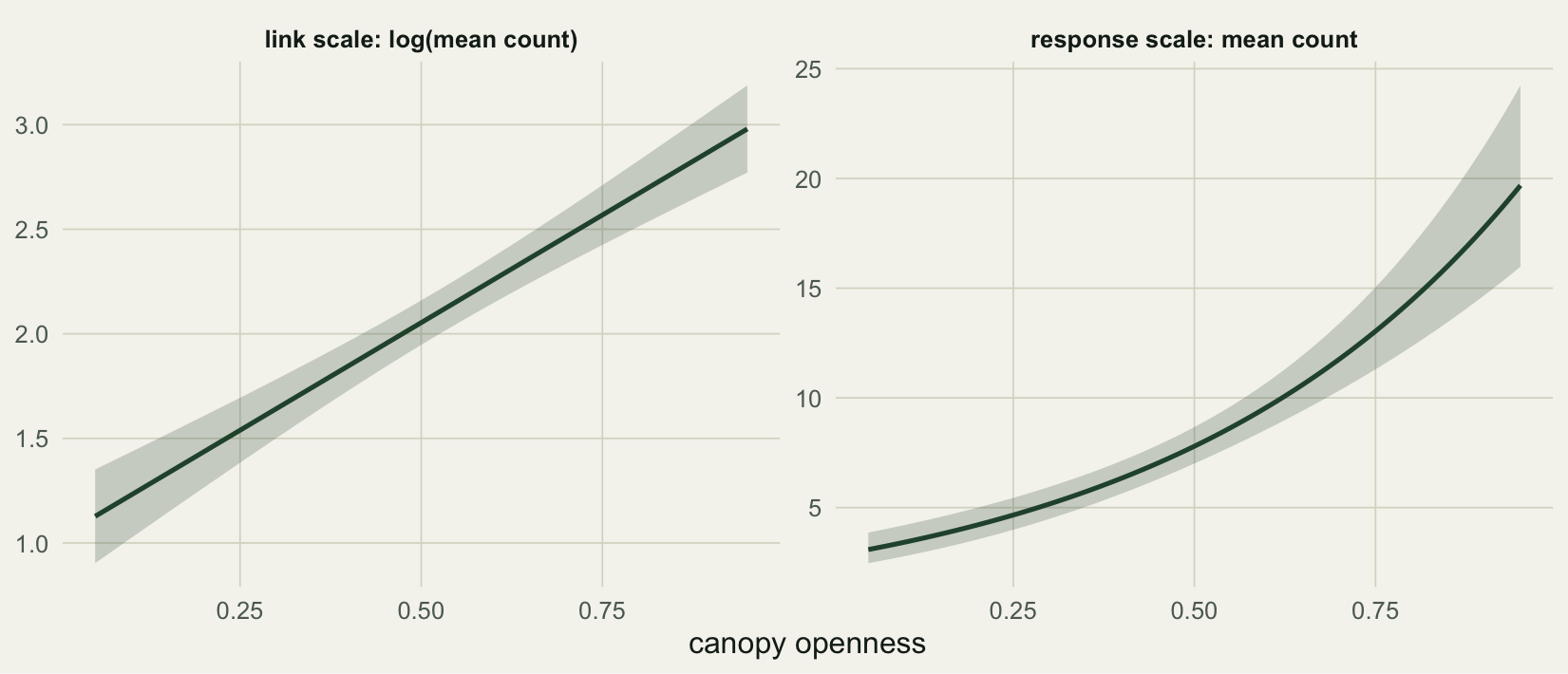
Plotting the same prediction on both scales shows what the inverse link does to the interval. On the log scale the line is straight and the band is an even ribbon. On the count scale the line bends upward and the band becomes lopsided: tighter below the curve, wider above it.
```{r}
#| label: fig-link-response
#| fig-cap: "The fitted canopy effect on the link scale (left) and the response scale (right), with elevation held at its mean. A symmetric interval on the left maps to a lopsided one on the right."
#| fig-alt: "Two panels. Left, on the log scale, a straight line with a band of even width. Right, on the count scale, an upward-bending curve whose band is narrow below and wide above."
#| fig-width: 8.6
#| fig-height: 3.7
two <- rbind(
  data.frame(canopy=grid$canopy, fit=pl$fit, lo=pl$fit-crit*pl$se.fit,
             hi=pl$fit+crit*pl$se.fit, scale="link scale: log(mean count)"),
  data.frame(canopy=grid$canopy, fit=grid$mu, lo=grid$lo, hi=grid$hi,
             scale="response scale: mean count"))
two$scale <- factor(two$scale, levels=unique(two$scale))
ggplot(two, aes(canopy, fit)) +
  geom_ribbon(aes(ymin=lo, ymax=hi), fill=forest, alpha=.22) +
  geom_line(colour=forest, linewidth=.9) +
  facet_wrap(~scale, scales="free_y") +
  labs(x="canopy openness", y=NULL) +
  theme_te()
```
The asymmetry is not a quirk of the plot; it is the honest shape of the interval. A 95% interval for the log mean is symmetric, and the exponential of a symmetric interval is not symmetric. Reporting `predicted +/- something` on the count scale throws that shape away.
## Why the symmetric shortcut misbehaves
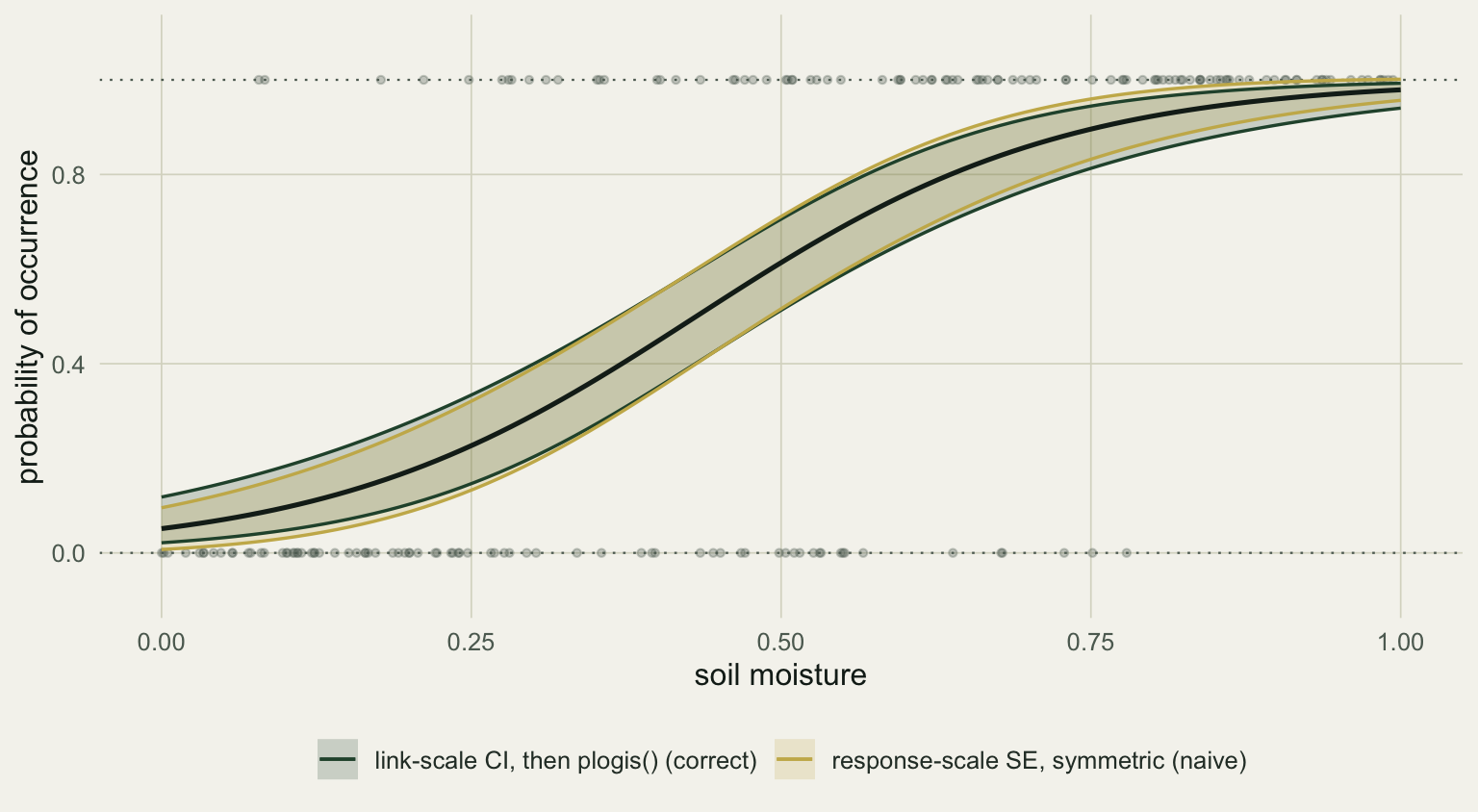
The shortcut is to ask `predict()` for the response scale directly and draw `fit +/- 1.96 * se`. Because the standard error is now on the response scale and the band is forced symmetric, it is not held inside the range of the response. A logistic model of occurrence makes this visible: near the top of the gradient the symmetric upper limit pushes past a probability of 1, which is not a probability at all.
```{r}
#| label: logistic
set.seed(206)
nb_   <- 180
moist <- runif(nb_, 0, 1)
occ   <- rbinom(nb_, 1, plogis(-2.5 + 6.0 * moist))
ml    <- glm(occ ~ moist, family = binomial)

gl  <- data.frame(moist = seq(0, 1, length.out = 100))
plk <- predict(ml, gl, type = "link",     se.fit = TRUE)
prr <- predict(ml, gl, type = "response", se.fit = TRUE)
gl$p   <- plogis(plk$fit)
gl$loc <- plogis(plk$fit - crit * plk$se.fit)   # correct: link CI, then plogis
gl$hic <- plogis(plk$fit + crit * plk$se.fit)
gl$lon <- prr$fit - crit * prr$se.fit           # naive: symmetric on response
gl$hin <- prr$fit + crit * prr$se.fit
c(naive_points_above_1 = sum(gl$hin > 1), max_naive_upper = round(max(gl$hin), 3))
```
```{r}
#| label: fig-boundary
#| fig-cap: "Predicted probability of occurrence with two bands. The link-scale band (forest) stays inside zero and one; the symmetric response-scale band (gold) leaks past both bounds."
#| fig-alt: "A logistic curve from low to high probability. A gold band crosses above the dotted line at probability one near the high end and below zero at the low end, while a forest band stays within the bounds."
#| fig-width: 8.0
#| fig-height: 4.4
bandb <- rbind(
  data.frame(moist=gl$moist, lo=gl$loc, hi=gl$hic, kind="link-scale CI, then plogis() (correct)"),
  data.frame(moist=gl$moist, lo=gl$lon, hi=gl$hin, kind="response-scale SE, symmetric (naive)"))
ggplot() +
  geom_hline(yintercept=c(0,1), colour=faint, linewidth=.4, linetype="dotted") +
  geom_point(data=data.frame(moist,occ), aes(moist, occ), colour=faint, alpha=.3, size=1.1) +
  geom_ribbon(data=bandb, aes(moist, ymin=lo, ymax=hi, fill=kind), alpha=.20) +
  geom_line(data=bandb, aes(moist, hi, colour=kind), linewidth=.6) +
  geom_line(data=bandb, aes(moist, lo, colour=kind), linewidth=.6) +
  geom_line(data=gl, aes(moist, p), colour=ink, linewidth=.9) +
  scale_fill_manual(values=c(forest, gold)) +
  scale_colour_manual(values=c(forest, gold)) +
  coord_cartesian(ylim=c(-0.08, 1.08)) +
  labs(x="soil moisture", y="probability of occurrence", fill=NULL, colour=NULL) +
  theme_te()
```
The overshoot here is small, only a little past 1, and that is itself worth understanding. A binomial variance shrinks as the probability approaches zero or one, so the symmetric band is least wrong exactly at the bounds and most wrong through the middle of the gradient, where the two bands separate the furthest. A count band behaves the same way: where the predicted mean is low the variance is low too, so the symmetric band rarely dips below zero, but it is still the wrong shape everywhere. The link-scale route sidesteps all of this for free.
## Marginal predictions: hold the other predictors somewhere
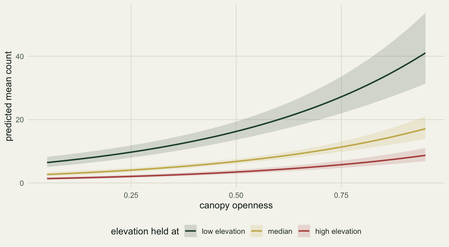
The grid above fixed `elev_z` at zero, its mean. That choice is part of the prediction, not a detail. To show the canopy effect you vary canopy and hold every other predictor at a representative value: the mean or median for a covariate, a chosen level for a factor (Fox 2003). Holding elevation at its tenth, fiftieth, and ninetieth percentile gives three versions of the same canopy curve, shifted up or down by the covariate.
```{r}
#| label: fig-conditioning
#| fig-cap: "The fitted canopy effect with elevation held at three values. The shape is the same; the covariate shifts the whole curve."
#| fig-alt: "Three upward curves of predicted count against canopy openness, one each for low, median, and high elevation, with the low-elevation curve highest."
#| fig-width: 8.0
#| fig-height: 4.4
elev_levels <- unname(quantile(dat$elev_z, c(0.1, 0.5, 0.9)))
elev_lab    <- c("low elevation","median","high elevation")
cond <- do.call(rbind, lapply(seq_along(elev_levels), function(k){
  g <- data.frame(canopy = seq(0.05, 0.95, length.out = 100), elev_z = elev_levels[k])
  p <- predict(m, newdata = g, type = "link", se.fit = TRUE)
  data.frame(canopy=g$canopy, elev_set=elev_lab[k], mu=exp(p$fit),
             lo=exp(p$fit-crit*p$se.fit), hi=exp(p$fit+crit*p$se.fit))
}))
cond$elev_set <- factor(cond$elev_set, levels=elev_lab)
ggplot(cond, aes(canopy, mu, colour=elev_set, fill=elev_set)) +
  geom_ribbon(aes(ymin=lo, ymax=hi), alpha=.16, colour=NA) +
  geom_line(linewidth=.9) +
  scale_colour_manual(values=c(forest, gold, "#b5534e")) +
  scale_fill_manual(values=c(forest, gold, "#b5534e")) +
  labs(x="canopy openness", y="predicted mean count",
       colour="elevation held at", fill="elevation held at") +
  theme_te()
```
At a canopy openness of 0.5 the predicted count runs from about 16 at low elevation to about 3.5 at high elevation. None of those numbers is "the" prediction; each is a prediction conditional on where you parked the covariate, which is why the held value belongs in the figure caption.
## Reading the slope: multiplicative, not additive
On the response scale a log-link effect is multiplicative. Exponentiating the coefficients gives those factors, with Wald intervals:
```{r}
#| label: exp-coef
round(exp(cbind(estimate = coef(m), confint.default(m))), 2)
```
The exponentiated canopy coefficient, 7.83, is the factor by which the mean count multiplies per unit of canopy; per 0.1 of canopy the factor is `exp(0.1 * 2.06)`, about 1.23, and it is the same factor everywhere along the gradient.
```{r}
#| label: multiplicative
g2 <- data.frame(canopy = c(0.3, 0.4, 0.7, 0.8), elev_z = 0)
p2 <- predict(m, newdata = g2, type = "response")
c(ratio_0.3_to_0.4 = unname(round(p2[2]/p2[1], 3)),
  ratio_0.7_to_0.8 = unname(round(p2[4]/p2[3], 3)),
  jump_0.3_to_0.4  = unname(round(p2[2]-p2[1], 2)),
  jump_0.7_to_0.8  = unname(round(p2[4]-p2[3], 2)))
```
The ratio is constant at 1.23, but the absolute change is not: moving canopy from 0.3 to 0.4 adds about one individual, while the same step from 0.7 to 0.8 adds nearly three. That is why a single sentence like "canopy adds N individuals" has no fixed answer on the count scale, and why the predicted curve, not a lone coefficient, is the honest summary.
## What the band does and does not cover
The interval here is for the mean count at a given canopy and elevation, not a prediction interval for a new plot. Individual plots scatter around the mean by the full negative binomial variance, which is much wider; if you need to bracket a future observation, simulate from the fitted model instead of widening this band. Two more limits worth stating: the held values are a choice, so report them, and the prediction has no anchor outside the range of the data, so do not read the curve past where canopy was actually sampled.
In practice you will reach for a helper rather than hand-building grids every time. The `effects` package (Fox 2003) and `ggeffects` (Ludecke 2018) compute adjusted predictions on the response scale, holding non-focal predictors at means or representative values, and return tidy frames ready for `ggplot2`; `marginaleffects` does the same and adds contrasts. The mechanics above are what those packages run underneath, which is the part worth seeing once before you let a function do it. The companion to this is checking that the model is worth predicting from at all: [residual diagnostics for GLMs](../glm-residual-diagnostics/).
## References
Fox J (2003). Effect Displays in R for Generalised Linear Models. *Journal of Statistical Software* 8(15):1-27. doi:10.18637/jss.v008.i15
Ludecke D (2018). ggeffects: Tidy Data Frames of Marginal Effects from Regression Models. *Journal of Open Source Software* 3(26):772. doi:10.21105/joss.00772
McCullagh P, Nelder JA (1989). *Generalized Linear Models*, 2nd ed. Chapman and Hall. ISBN 0-412-31760-5
Nelder JA, Wedderburn RWM (1972). Generalized Linear Models. *Journal of the Royal Statistical Society A* 135(3):370-384. doi:10.2307/2344614
Bolker BM (2008). *Ecological Models and Data in R*. Princeton University Press. ISBN 978-0-691-12522-0