A particle filter for animal movement

Build a bootstrap particle filter from scratch in base R for animal tracks with heavy-tailed Argos errors, where the Gaussian Kalman filter is dragged off course by outliers.

The Kalman filter is exact, fast, and completely dependent on one assumption: Gaussian observation error. Location data often break it. Argos fixes in particular throw the occasional gross outlier, a position hundreds of metres from the truth, and a least-squares filter chases those outliers because a Gaussian likelihood treats a far-off point as almost impossible and so heaves the estimate toward it. The remedy is a heavier-tailed observation model, which no longer has a closed form. A particle filter handles it by brute force: represent the belief about the animal’s state with a cloud of weighted samples, push them through the movement model, and reweight by how well each explains the next fix. This post codes a bootstrap particle filter from scratch and shows it shrugging off outliers that drag the Kalman filter off course.

Contaminated observations

We keep the correlated random walk movement process from the earlier post, but corrupt the observations: most carry ordinary Gaussian error, and a minority are gross outliers with a far larger spread. This contaminated model is a standard stand-in for Argos error.

set.seed(2207)
n<-300; gamma_t<-0.6; sigma_t<-5; tau_t<-5; p_out<-0.12; k_out<-7
vx<-vy<-numeric(n)
vx[1]<-rnorm(1,0,sigma_t/sqrt(1-gamma_t^2)); vy[1]<-rnorm(1,0,sigma_t/sqrt(1-gamma_t^2))
for(t in 2:n){ vx[t]<-gamma_t*vx[t-1]+rnorm(1,0,sigma_t); vy[t]<-gamma_t*vy[t-1]+rnorm(1,0,sigma_t) }
px<-cumsum(vx); py<-cumsum(vy)
out<-rbinom(n,1,p_out)                          # which fixes are gross outliers
sdv<-ifelse(out==1, k_out*tau_t, tau_t)
ox<-px+rnorm(n,0,sdv); oy<-py+rnorm(n,0,sdv)
n_out<-sum(out); worst<-max(sqrt((ox-px)^2+(oy-py)^2))
c(n=n, outliers=n_out, worst_error=round(worst))

          n    outliers worst_error 
        300          39          81 

Of the 300 fixes, 39 are gross outliers, and the worst sits 81 metres from the truth.

The Gaussian filter, and why it fails here

First the baseline: fit the linear-Gaussian model of the earlier post by maximum likelihood and filter with it. The estimated observation error inflates as the Gaussian model stretches to accommodate the outliers, and the filtered track still lurches toward them.

kf_coord<-function(y,g,s2,h2){
  n<-length(y); Tm<-matrix(c(1,0,g,g),2,2); Q<-s2*matrix(c(1,1,1,1),2,2); Z<-matrix(c(1,0),1,2)
  a<-c(y[1],0); P<-matrix(c(h2,0,0,s2/(1-g^2)),2,2); ll<-0; af<-matrix(NA,n,2); af[1,]<-a
  for(t in 2:n){ ap<-as.vector(Tm%*%a); Pp<-Tm%*%P%*%t(Tm)+Q
    v<-y[t]-as.vector(Z%*%ap); Ft<-as.vector(Z%*%Pp%*%t(Z))+h2; K<-as.vector(Pp%*%t(Z))/Ft
    a<-ap+K*v; P<-Pp-(K%*%Z)%*%Pp; ll<-ll-0.5*(log(2*pi)+log(Ft)+v^2/Ft); af[t,]<-a }
  list(ll=ll, p=af[,1]) }
nll<-function(par){g<-plogis(par[1]);s2<-exp(par[2]);h2<-exp(par[3])
  -(kf_coord(ox,g,s2,h2)$ll+kf_coord(oy,g,s2,h2)$ll)}
fk<-optim(c(qlogis(.5),log(25),log(25)),nll,method="Nelder-Mead",control=list(reltol=1e-10,maxit=3000))
gk<-plogis(fk$par[1]); s2k<-exp(fk$par[2]); h2k<-exp(fk$par[3])
kfx<-kf_coord(ox,gk,s2k,h2k)$p; kfy<-kf_coord(oy,gk,s2k,h2k)$p
c(gamma=round(gk,3), sigma=round(sqrt(s2k),2), tau=round(sqrt(h2k),2))

 gamma  sigma    tau 
 0.511  5.370 12.340 

The observation standard deviation is estimated at 12.34, well above the true core value of 5, because the Gaussian model can only explain the outliers by assuming all fixes are noisier than they are.

A bootstrap particle filter, by hand

The particle filter represents the state distribution with 5000 particles. At each step it moves every particle through the movement model, then weights it by a heavy-tailed observation density, here a Student-t, which assigns a far-off fix a small but not vanishing likelihood, so an outlier no longer commands the estimate. Weights concentrate over time, so we monitor the effective sample size and resample when it falls below half the particle count. Resampling with a systematic scheme keeps the cloud healthy.

systematic_resample<-function(w){
  N<-length(w); pos<-(runif(1)+0:(N-1))/N; cw<-cumsum(w); idx<-integer(N); j<-1
  for(i in 1:N){ while(cw[j]<pos[i]) j<-j+1; idx[i]<-j }; idx }

run_pf<-function(nu, resample=TRUE, N=5000, seed=99){
  set.seed(seed)
  g<-gamma_t; s<-sigma_t; sc<-tau_t                 # process at truth; obs model = t_nu(scale sc)
  Px<-matrix(0,N,4)                                 # columns: px, vx, py, vy
  Px[,2]<-rnorm(N,0,s/sqrt(1-g^2)); Px[,4]<-rnorm(N,0,s/sqrt(1-g^2))
  Px[,1]<-ox[1]+rnorm(N,0,sc); Px[,3]<-oy[1]+rnorm(N,0,sc)
  w<-rep(1/N,N); est<-matrix(NA,n,2); ess<-numeric(n)
  est[1,]<-c(weighted.mean(Px[,1],w), weighted.mean(Px[,3],w)); ess[1]<-1/sum(w^2)
  for(t in 2:n){
    Px[,2]<-g*Px[,2]+rnorm(N,0,s); Px[,1]<-Px[,1]+Px[,2]     # propagate
    Px[,4]<-g*Px[,4]+rnorm(N,0,s); Px[,3]<-Px[,3]+Px[,4]
    ld<-dt((ox[t]-Px[,1])/sc,df=nu,log=TRUE)-log(sc)+
        dt((oy[t]-Px[,3])/sc,df=nu,log=TRUE)-log(sc)         # heavy-tailed weights
    lw<-log(w)+ld; lw<-lw-max(lw); w<-exp(lw); w<-w/sum(w)
    est[t,]<-c(sum(w*Px[,1]), sum(w*Px[,3])); ess[t]<-1/sum(w^2)
    if(resample && ess[t]<N/2){ idx<-systematic_resample(w); Px<-Px[idx,]; w<-rep(1/N,N) }
  }
  list(px=est[,1], py=est[,2], ess=ess) }

pf      <- run_pf(nu=4, resample=TRUE)
pf_nores<- run_pf(nu=4, resample=FALSE)

rmse<-function(ex,ey) sqrt(mean((ex-px)^2+(ey-py)^2))
rmse_obs<-rmse(ox,oy); rmse_kf<-rmse(kfx,kfy); rmse_pf<-rmse(pf$px,pf$py)
ess_med<-median(pf$ess); n_res<-sum(pf$ess<5000/2)
collapse<-which(pf_nores$ess<10)[1]
c(rmse_obs=round(rmse_obs,2), rmse_kf=round(rmse_kf,2), rmse_pf=round(rmse_pf,2))

rmse_obs  rmse_kf  rmse_pf 
   17.82    11.85     9.31 

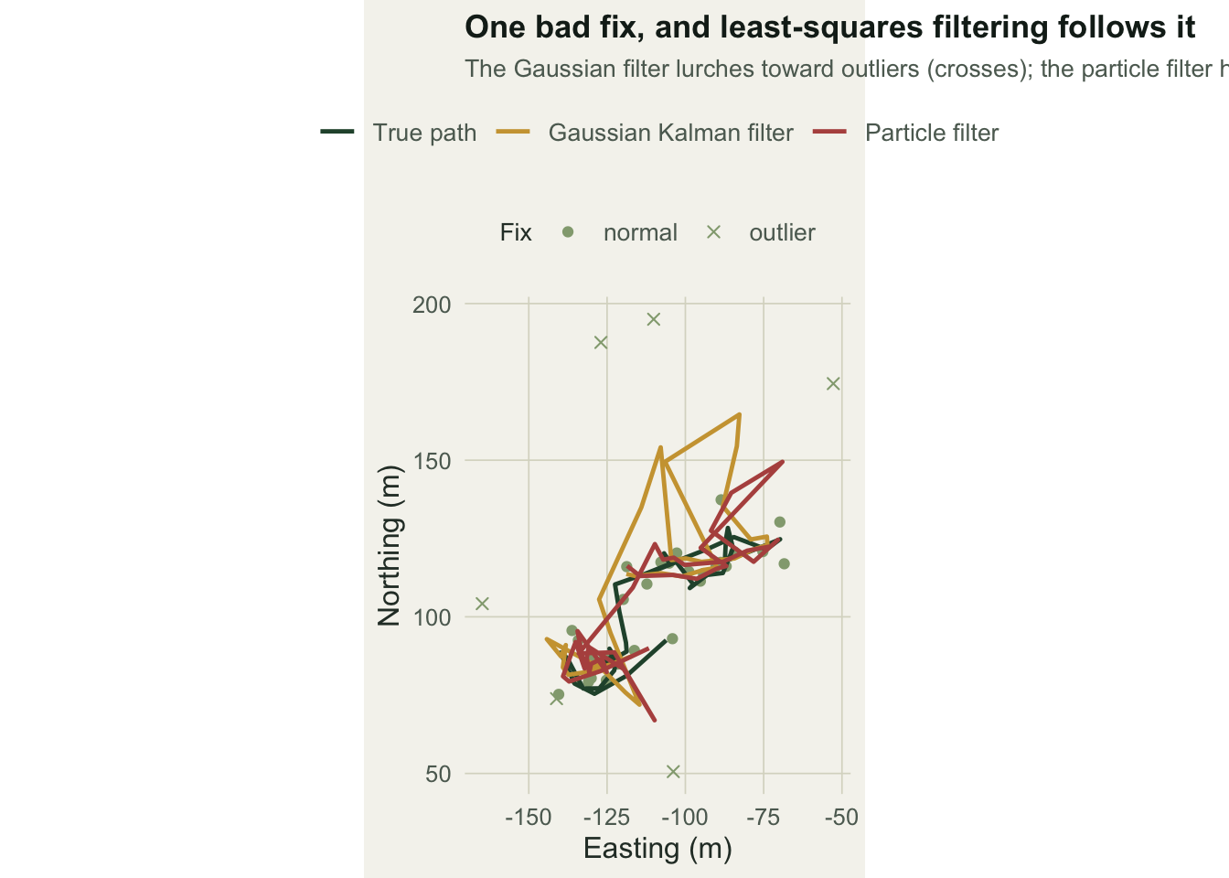
The heavy-tailed particle filter sits 9.31 metres from the true path on average, against 11.85 for the Gaussian Kalman filter and 17.82 for the raw fixes. Trusting the outliers less, not more, is what buys the improvement.

Figure 1: A window around the worst outlier. The Gaussian filter (gold) lurches toward the stray fixes (crosses); the particle filter (red) holds close to the truth (green).

Why resampling is not optional

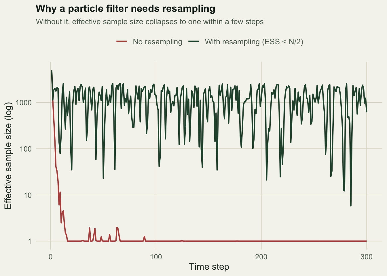
A particle filter without resampling degenerates: after a few steps one particle carries almost all the weight and the cloud is dead. Tracking the effective sample size makes this concrete.

Figure 2: Effective sample size over time, with and without resampling. Without it, the effective sample size collapses to one within a few steps.

With adaptive resampling the effective sample size holds at a median of about 1238 of the 5000 particles, triggering a resample at 291 of the 300 steps. Without resampling it drops below ten by step 8 and never recovers. The bootstrap filter is simple to write, but this diagnostic is the price of admission: always watch the effective sample size, and resample before the cloud collapses.

Where this fits

The particle filter buys tolerance of non-Gaussian error at the cost of speed and of Monte Carlo noise, and it needs enough particles that the estimates settle. For a linear-Gaussian problem the Kalman filter of the earlier posts is exact and far cheaper, so reach for particles only when the observation model genuinely demands it, as heavy-tailed Argos error does. The common thread across the batch holds once more: the raw fixes mislead, and a filter is only as good as the error model you give it.

References

Gordon, Salmond and Smith 1993. IEE Proceedings F 140(2):107-113 (10.1049/ip-f-2.1993.0015)

Patterson, Thomas, Wilcox, Ovaskainen and Matthiopoulos 2008. Trends in Ecology and Evolution 23(2):87-94 (10.1016/j.tree.2007.10.009)

Jonsen, Flemming and Myers 2005. Ecology 86(11):2874-2880 (10.1890/04-1852)

Kalman 1960. Journal of Basic Engineering 82(1):35-45 (10.1115/1.3662552)

Auger-Methe, Newman, Cole, Empacher, Gryba, King, Leos-Barajas, Mills Flemming, Nielsen, Petris and Thomas 2021. Ecological Monographs 91(4):e01470 (10.1002/ecm.1470)

Related tutorials

• State-space models for animal movement
• A Gompertz state-space model
• Correlated random walks and movement
• Fitting a two-state movement HMM