Occupancy and detection covariates in R

Let occupancy depend on habitat and detection on survey effort in a single-season occupancy model, then predict occupancy with confidence bands in base R.

A constant occupancy and a constant detection probability answer only the plainest question: how much of the landscape is occupied, on average. The interesting questions are conditional. Does this species favour wetter sites? Do longer surveys find it more often? An occupancy model earns its place once occupancy is allowed to track habitat and detection is allowed to track survey effort, each on its own scale.

This post extends the hand-written single-season likelihood so that occupancy and detection each carry their own linear predictor. The mechanics are a short step from the constant-parameter version, and the payoff is a fitted occupancy curve with an honest confidence band. Everything runs in base R with optim.

Two processes, two covariates

We simulate 300 sites with five visits each. Occupancy rises with a standardised habitat covariate, while per-visit detection rises with a standardised measure of survey effort. Both covariates act on the logit scale, so the true relationships are logit(psi) = -0.3 + 1.4 * habitat and logit(p) = -0.2 + 0.7 * effort.

set.seed(101)
R <- 300L; K <- 5L
habitat <- as.numeric(scale(rnorm(R)))
effort  <- as.numeric(scale(runif(R, 1, 5)))
a_true <- c(-0.3, 1.4)          # occupancy intercept and habitat slope
b_true <- c(-0.2, 0.7)          # detection intercept and effort slope
psi_i <- plogis(a_true[1] + a_true[2] * habitat)
p_i   <- plogis(b_true[1] + b_true[2] * effort)
z <- rbinom(R, 1, psi_i)
y <- matrix(rbinom(R * K, 1, rep(z, K) * rep(p_i, K)), R, K)
d <- rowSums(y)
c(realised_occ = round(mean(z), 3), naive_detrate = round(mean(d >= 1), 3))

 realised_occ naive_detrate 
        0.477         0.423 

Realised occupancy is 0.477, while the naive detected-site rate is 0.423. Detection varies from site to site here, since effort does, so p_i stays high enough at most sites for the repeat visits to remain informative.

Adding the linear predictors

The likelihood keeps the two-case structure from the constant model, but now psi and p are vectors, one value per site, built from design matrices. The occupancy design matrix holds an intercept and habitat; the detection design matrix holds an intercept and effort. The parameter vector stacks the two sets of coefficients, and optim estimates all four together.

X <- cbind(1, habitat)          # occupancy design matrix
W <- cbind(1, effort)           # detection design matrix
nll <- function(par, y, K, X, W) {
  a <- par[1:ncol(X)]
  b <- par[(ncol(X) + 1):(ncol(X) + ncol(W))]
  psi <- plogis(as.vector(X %*% a))
  p   <- plogis(as.vector(W %*% b))
  d <- rowSums(y)
  lik <- ifelse(d > 0, psi * p^d * (1 - p)^(K - d), psi * (1 - p)^K + (1 - psi))
  -sum(log(lik))
}
fit <- optim(rep(0, 4), nll, y = y, K = K, X = X, W = W, method = "BFGS", hessian = TRUE)
V <- solve(fit$hessian); se <- sqrt(diag(V)); est <- fit$par
res <- data.frame(term = c("psi_int", "psi_habitat", "p_int", "p_effort"),
                  estimate = round(est, 3), se = round(se, 3), truth = c(a_true, b_true))
res

         term estimate    se truth
1     psi_int   -0.219 0.154  -0.3
2 psi_habitat    1.421 0.205   1.4
3       p_int   -0.143 0.092  -0.2
4    p_effort    0.709 0.095   0.7

The occupancy slope on habitat is estimated at 1.421 with a standard error of 0.205, close to the true 1.4, and the detection slope on effort at 0.709 against a true 0.7. Both intercepts land near their targets as well. The model has separated a habitat effect on where the species lives from an effort effect on whether it was seen, using nothing but the detection histories.

Why not just regress the raw detections?

A tempting shortcut is to run an ordinary logistic regression of “detected at least once” on habitat and skip the detection process entirely. It gives a habitat slope, but a biased one.

naive_glm <- glm((d >= 1) ~ habitat, family = binomial)
round(coef(naive_glm)[["habitat"]], 3)

[1] 1.28

The naive slope is 1.28, pulled in from the true 1.4. Imperfect detection attenuates the estimated habitat effect, because missed detections blur the contrast between good and poor sites: some good sites record a blank, some poor sites happen to be occupied and detected, and the gradient flattens. The occupancy model, which models the missing detections explicitly, does not suffer this shrinkage.

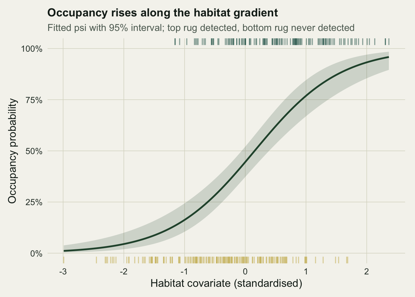
Predicting occupancy along the gradient

The point of fitting covariates is to read off the fitted relationship. The right way to attach uncertainty is to work on the linear-predictor scale, where the model is linear and the sampling distribution is roughly symmetric, then transform the endpoints back with plogis. Building the interval directly on the probability scale would misbehave near zero and one.

hx <- seq(min(habitat), max(habitat), length.out = 100)
Xg <- cbind(1, hx); Va <- V[1:2, 1:2]
eta <- as.vector(Xg %*% est[1:2])
se_eta <- sqrt(rowSums((Xg %*% Va) * Xg))          # delta-method SE on the logit scale
band <- data.frame(hx = hx, psi = plogis(eta),
                   lo = plogis(eta - 1.96 * se_eta),
                   hi = plogis(eta + 1.96 * se_eta))
rug <- data.frame(habitat = habitat, det = ifelse(d >= 1, 1, 0))
ggplot(band, aes(hx, psi)) +
  geom_ribbon(aes(ymin = lo, ymax = hi), fill = te_forest, alpha = 0.18) +
  geom_line(colour = te_forest, linewidth = 1) +
  geom_rug(data = subset(rug, det == 1), aes(x = habitat), inherit.aes = FALSE,
           sides = "t", colour = te_deep, alpha = 0.5, length = unit(0.03, "npc")) +
  geom_rug(data = subset(rug, det == 0), aes(x = habitat), inherit.aes = FALSE,
           sides = "b", colour = te_gold, alpha = 0.5, length = unit(0.03, "npc")) +
  scale_y_continuous(limits = c(0, 1), labels = scales::percent_format(1)) +
  labs(title = "Occupancy rises along the habitat gradient",
       subtitle = "Fitted psi with 95% interval; top rug detected, bottom rug never detected",
       x = "Habitat covariate (standardised)", y = "Occupancy probability") +
  theme_te(13)

Figure 1: Fitted occupancy against the habitat covariate with a 95 per cent confidence band. Top rug marks sites detected at least once; bottom rug marks sites never detected.

Reading the curve at three points makes the gradient concrete: predicted occupancy climbs from about 0.045 at two standard deviations below average habitat, through 0.446 at the mean, to 0.932 two standard deviations above. At the mean the band is tight, with a half-width near 0.074, and it widens towards the sparsely sampled ends of the gradient, as an honest interval should.

round(plogis(est[1] + est[2] * c(-2, 0, 2)), 3)   # psi at habitat -2, 0, +2

[1] 0.045 0.446 0.932

i0 <- which.min(abs(hx))
round((band$hi[i0] - band$lo[i0]) / 2, 3)          # CI half-width at mean habitat

[1] 0.074

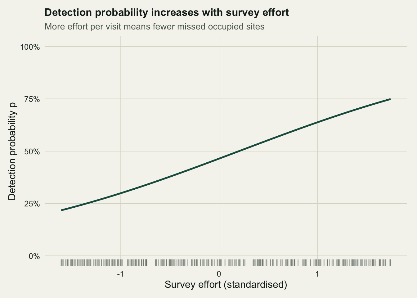
Detection responds to effort

The detection side of the model tells its own story. Holding the occupancy process aside, per-visit detection climbs with survey effort, so the same site is likelier to yield a detection when more time or a longer transect goes into each visit.

ex <- seq(min(effort), max(effort), length.out = 100)
pdet <- data.frame(ex = ex, p = plogis(est[3] + est[4] * ex))
ggplot(pdet, aes(ex, p)) +
  geom_line(colour = te_deep, linewidth = 1) +
  geom_rug(data = data.frame(effort = effort), aes(x = effort), inherit.aes = FALSE,
           sides = "b", colour = te_faint, alpha = 0.4) +
  scale_y_continuous(limits = c(0, 1), labels = scales::percent_format(1)) +
  labs(title = "Detection probability increases with survey effort",
       subtitle = "More effort per visit means fewer missed occupied sites",
       x = "Survey effort (standardised)", y = "Detection probability p") +
  theme_te(12)

Figure 2: Fitted per-visit detection probability against survey effort. More effort per visit means fewer occupied sites slip through unrecorded.

Detection runs from about 0.231 at low effort to 0.715 at high effort across the sampled range. The practical reading is direct: where effort is thin, the detection process is doing more of the work in the likelihood, and occupancy at those sites rests on a shakier footing. It is a reminder that the two curves are not independent stories but two halves of the same accounting.

round(plogis(est[3] + est[4] * c(-1.5, 1.5)), 3)   # p at effort -1.5, +1.5

[1] 0.231 0.715

Reading the model well

A few habits keep covariate occupancy models honest. Standardise the covariates before fitting, as here, so the intercept means occupancy and detection at average conditions and the slopes are comparable in size. Keep the occupancy and detection covariates conceptually separate: habitat belongs to where the species lives, effort to whether you saw it, and mixing them invites the model to explain a detection shortfall as a real absence. Read effects through predictions on the response scale, with intervals built on the linear predictor, rather than eyeballing the raw coefficients. With those in place, the fitted curves say what you want them to say, which is where the species is, corrected for the chance of missing it.

References

• MacKenzie D I, Nichols J D, Lachman G B, Droege S, Royle J A, Langtimm C A 2002 Ecology 83(8):2248-2255 (10.1890/0012-9658(2002)083[2248:ESORWD]2.0.CO;2)
• MacKenzie D I, Nichols J D, Royle J A, Pollock K H, Bailey L L, Hines J E 2018 Occupancy Estimation and Modeling, 2nd ed. Academic Press. ISBN 978-0-12-407197-1
• Kery M, Royle J A 2016 Applied Hierarchical Modeling in Ecology, Vol 1. Academic Press. ISBN 978-0-12-801378-6
• Fiske I, Chandler R B 2011 Journal of Statistical Software 43(10):1-23 (10.18637/jss.v043.i10)

Related tutorials

• Fitting single-season occupancy models in R
• Predicting from a GLM on the response scale
• Logistic regression for presence/absence data
• Species distribution modelling with GLM in R