library(ggplot2)
library(patchwork)

te_paper  <- "#f5f4ee"
te_ink    <- "#16241d"
te_body   <- "#2c3a31"
te_forest <- "#275139"
te_rust   <- "#b5534e"
te_gold   <- "#c9b458"
te_line   <- "#dad9ca"

theme_datasheet <- function() {
  theme_minimal(base_size = 12) +
    theme(plot.background  = element_rect(fill = te_paper, colour = NA),
          panel.background = element_rect(fill = te_paper, colour = NA),
          panel.grid.major = element_line(colour = te_line, linewidth = 0.3),
          panel.grid.minor = element_blank(),
          text             = element_text(colour = te_body),
          plot.title       = element_text(colour = te_ink, face = "bold"),
          plot.subtitle    = element_text(colour = te_body),
          axis.text        = element_text(colour = te_body))
}Neighbourhood colonisation and false jumps
R
occupancy
invasion
spatial
ecology tutorial
Imperfect detection invents long-distance jumps in a spreading grid. Simulate neighbourhood colonisation in R and compare three fits of the background rate.
A survey programme has a grid of tetrads and an invader moving through it. Each year a team visits every tetrad three times and records whether the species was found. After eight years somebody asks the question that decides the budget: of all the squares that were newly occupied, how many were filled from a neighbour and how many appeared out of nowhere. The first number argues for clearing the front. The second argues for sending people out to find and kill satellite colonies far ahead of it.
The grid answers that question badly, and it answers it badly twice over. Dynamic occupancy: colonisation and extinction has the first half already: a site you fail to detect this season is scored as an extinction, and when it turns up again next season it is scored as a colonisation, so naive turnover read off detections is not turnover. That post makes the point without space, on independent sites, and shows apparent colonisation biased far less than apparent extinction. Put the same sites on a grid and a second failure appears on top of the first. The non-detection that invents a colonisation at the focal square also happens at its neighbours, and a neighbour you did not detect cannot be credited as the source. The invented colonisation is therefore not merely invented; it is filed under the wrong heading.
That heading is a management quantity. Long-distance jumps and stratified spread prices the two options against each other in treated area and finds the crossover between clearing the front and hunting detached colonies at a founding rate that the programme has to estimate from its own data. This post is about the estimate, not the decision: what a survey grid says about the share of colonisations with no adjacent source, and what a model recovers.
The model side is not new. Bled, Royle and Cam fitted the spread of the Eurasian collared-dove with a colonisation probability built from latent neighbour states, and Yackulic and colleagues modelled barred owl colonisation as a function of neighbourhood occupancy in the Oregon Coast Ranges; Broms and colleagues set out the family of explicit colonisation processes these belong to, and write the colonisation probability as a product over the occupied neighbours. The product form used below, one minus the probability that every occupied neighbour failed to colonise, is the one Broms and colleagues use. What is measured here is what happens when you plug in the neighbour count you observed instead of estimating the latent one: how far the background rate is off, in which direction the per-neighbour effect moves, and what one smoothing pass buys. The last section adds a cost that is not a detection error at all, and that grows as the survey improves instead of shrinking with it.
The direction of the covariate error is worth flagging before the numbers arrive, because it is the opposite of the one most readers expect. Measurement error and regression dilution is the standard picture: a predictor measured with error pulls its own slope towards zero. The observed neighbour count is a predictor measured with error, so attenuation is the natural guess. It is not what happens here.
A grid where colonisation comes from next door
The truth is a two-state Markov chain on a square grid with rook adjacency, which is the dynamic occupancy model of MacKenzie and colleagues with one covariate on the colonisation probability: the number of occupied neighbours at the end of the previous season. An occupied site goes locally extinct with a fixed probability. An empty site is colonised with a probability written as a product, one minus the chance that the background failed and every occupied neighbour failed as well.
n_side  <- 25
n_site  <- n_side^2
n_season <- 8
n_visit  <- 3
g0_true  <- 0.01
gnb_true <- 0.25
eps_true <- 0.10

nb_count <- function(mat) {
  pad <- matrix(0, n_side + 2, n_side + 2)
  pad[2:(n_side + 1), 2:(n_side + 1)] <- mat
  pad[1:n_side, 2:(n_side + 1)] + pad[3:(n_side + 2), 2:(n_side + 1)] +
    pad[2:(n_side + 1), 1:n_side] + pad[2:(n_side + 1), 3:(n_side + 2)]
}

sim_grid <- function(p_det) {
  z <- array(0L, c(n_side, n_side, n_season))
  seed_block <- matrix(0L, n_side, n_side)
  seed_block[11:15, 11:15] <- 1L
  z[, , 1] <- seed_block
  for (t in 2:n_season) {
    k_occ <- nb_count(z[, , t - 1])
    gam   <- 1 - (1 - g0_true) * (1 - gnb_true)^k_occ
    z[, , t] <- ifelse(z[, , t - 1] == 1L,
                       rbinom(n_site, 1, 1 - eps_true),
                       rbinom(n_site, 1, gam))
  }
  y <- array(rbinom(n_site * n_season * n_visit, 1,
                    p_det * rep(as.vector(z), n_visit)),
             c(n_side, n_side, n_season, n_visit))
  list(z = z, det = apply(y, c(1, 2, 3), sum))
}

gam_true_k <- function(k) 1 - (1 - g0_true) * (1 - gnb_true)^k
gam_grid   <- gam_true_k(0:4)
Every constant in that chunk was fixed before anything was run and none of them was revised afterwards. The background colonisation probability is 0.01, the per-neighbour probability 0.25, the extinction probability 0.10. A site with one occupied neighbour is therefore colonised with probability 0.258, with two neighbours 0.443, and with all four 0.687. Spread is overwhelmingly local by construction: the background is 25 times smaller than the effect of a single neighbour, which is roughly the regime a manager cares about, because that is when the rare non-local event is worth chasing.
The grid is 25 by 25, run for 8 seasons with 3 visits per season, and starts from a five by five block of occupied sites in the middle. A jump is defined by the truth as a colonisation at a site with no occupied neighbour in the previous season. A naive analyst, treating detection as occupancy, defines it as an observed colonisation at a site with no observed occupied neighbour in the previous season. Those two definitions are the whole subject.
set.seed(6021)
p_show   <- 0.3
run_show <- sim_grid(p_show)
z_show   <- run_show$z
obs_show <- (run_show$det > 0) * 1L
t_show   <- 5

k_prev_true <- nb_count(z_show[, , t_show - 1])
k_prev_obs  <- nb_count(obs_show[, , t_show - 1])
col_true    <- z_show[, , t_show - 1] == 0 & z_show[, , t_show] == 1
col_obs     <- obs_show[, , t_show - 1] == 0 & obs_show[, , t_show] == 1

n_col_true  <- sum(col_true)
n_jump_true <- sum(col_true & k_prev_true == 0)
n_col_obs   <- sum(col_obs)
n_jump_obs  <- sum(col_obs & k_prev_obs == 0)
n_phantom   <- sum(col_obs & k_prev_obs == 0 & z_show[, , t_show - 1] == 1)
occ_share   <- mean(z_show[, , t_show - 1])
seen_share  <- mean(obs_show[, , t_show - 1])
In the single replicate drawn above, at a per-visit detection of 0.3, season 5 follows a season in which 0.123 of the grid was occupied and 0.067 of it was seen. The truth records 37 colonisations, of which 5 had no occupied neighbour. The survey records 48 colonisations, of which 24 had no observed occupied neighbour, and 10 of those 24 were at sites that were already occupied the year before.
grid_frame <- function(state_prev, colonised, k_prev, panel_lab) {
  idx <- expand.grid(x = 1:n_side, y = 1:n_side)
  base <- data.frame(idx,
                     prev = ifelse(as.vector(state_prev) == 1, "occupied", "empty"),
                     panel = panel_lab)
  pts <- data.frame(idx,
                    col = as.vector(colonised),
                    jump = as.vector(k_prev) == 0,
                    panel = panel_lab)
  pts <- pts[pts$col, ]
  pts$kind <- ifelse(pts$jump, "no source next door", "source next door")
  list(base = base, pts = pts)
}

fr_true <- grid_frame(z_show[, , t_show - 1], col_true, k_prev_true, "truth")
fr_obs  <- grid_frame(obs_show[, , t_show - 1], col_obs, k_prev_obs,
                      "what the survey recorded")

map_panel <- function(fr, sub_lab) {
  ggplot(fr$base, aes(x, y)) +
    geom_tile(aes(fill = prev), colour = te_paper, linewidth = 0.25) +
    geom_point(data = fr$pts, aes(colour = kind, shape = kind), size = 1.7,
               stroke = 0.7) +
    scale_fill_manual(values = c(empty = te_line, occupied = te_forest),
                      name = "state last season") +
    scale_colour_manual(values = c("source next door" = te_ink,
                                   "no source next door" = te_rust), name = NULL) +
    scale_shape_manual(values = c("source next door" = 16,
                                  "no source next door" = 1), name = NULL) +
    coord_equal(expand = FALSE) +
    labs(x = NULL, y = NULL, title = fr$base$panel[1], subtitle = sub_lab) +
    theme_datasheet() +
    theme(axis.text = element_blank(), panel.grid = element_blank(),
          legend.position = "bottom", legend.box = "vertical",
          legend.margin = margin(0, 0, 0, 0))
}

(map_panel(fr_true, sprintf("%d colonisations, %d with no source",
                            n_col_true, n_jump_true)) +
 map_panel(fr_obs, sprintf("%d colonisations, %d scored as jumps",
                           n_col_obs, n_jump_obs))) +
  plot_layout(guides = "collect") +
  plot_annotation(theme = theme_datasheet()) &
  theme(legend.position = "bottom")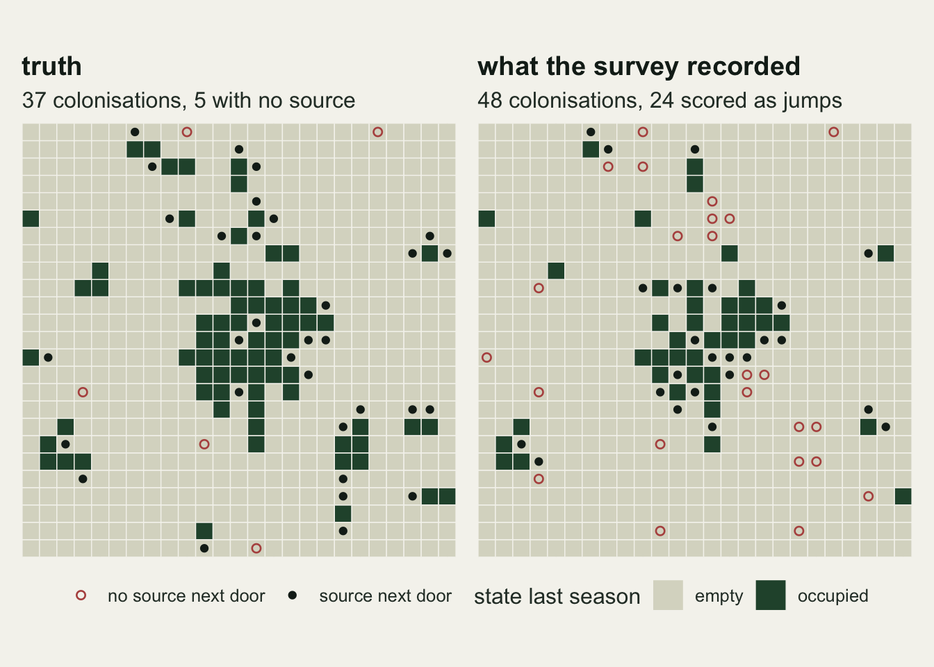
The right panel is the whole mechanism in one picture. The occupied field has been shot full of holes by non-detection, so sites inside it look empty, and when they are seen again they look like arrivals. The same holes remove the neighbours that would have explained those arrivals, so the arrivals look unexplained.
The false jump rate is almost closed form
Before any model is fitted, the size of the naive error can be written down. Let q be the probability that a truly occupied site is missed on all visits in a season, so that q is one minus the detection probability, raised to the number of visits. Conditional on the true state sequence, every detection event is independent, and the three things a naive jump requires can be multiplied.
A site is scored as a colonisation in season t when it is detected in t, which requires it to be truly occupied and needs probability one minus q, and when it was not detected in season t minus one, which has probability q if the site was truly occupied then and probability one otherwise. It is scored as a jump when none of its truly occupied neighbours was detected in season t minus one, which has probability q raised to the number of those neighbours. The denominator of the naive background rate counts sites that looked empty and had no visible occupied neighbour, which is the same two factors without the detection in t.
naive_pieces <- function(z_arr, det_arr, p_det) {
  q_miss <- (1 - p_det)^n_visit
  obs <- (det_arr > 0) * 1L
  num_o <- den_o <- num_t <- den_t <- 0
  e_num <- e_den <- e_col <- e_jump <- 0
  for (t in 2:n_season) {
    k_true <- nb_count(z_arr[, , t - 1])
    k_obs  <- nb_count(obs[, , t - 1])
    c_true <- z_arr[, , t - 1] == 0 & z_arr[, , t] == 1
    c_obs  <- obs[, , t - 1] == 0 & obs[, , t] == 1
    num_o  <- num_o + sum(c_obs & k_obs == 0)
    den_o  <- den_o + sum(obs[, , t - 1] == 0 & k_obs == 0)
    num_t  <- num_t + sum(c_true & k_true == 0)
    den_t  <- den_t + sum(z_arr[, , t - 1] == 0 & k_true == 0)
    w_look <- q_miss^(z_arr[, , t - 1]) * q_miss^k_true
    e_num  <- e_num + sum((z_arr[, , t] == 1) * (1 - q_miss) * w_look)
    e_den  <- e_den + sum(w_look)
    e_col  <- e_col + sum((z_arr[, , t] == 1) * (1 - q_miss) *
                            q_miss^(z_arr[, , t - 1]))
    e_jump <- e_jump + sum((z_arr[, , t] == 1) * (1 - q_miss) *
                             q_miss^(z_arr[, , t - 1]) * q_miss^k_true)
  }
  c(g0_naive = num_o / den_o, g0_exp = e_num / e_den,
    g0_truth = num_t / den_t, jump_exp = e_jump / e_col,
    q_miss = q_miss)
}

check_show <- naive_pieces(z_show, run_show$det, p_show)
jump_obs_all <- {
  obs_all <- (run_show$det > 0) * 1L
  nj <- nc <- 0
  for (t in 2:n_season) {
    k_obs  <- nb_count(obs_all[, , t - 1])
    c_obs  <- obs_all[, , t - 1] == 0 & obs_all[, , t] == 1
    nc <- nc + sum(c_obs); nj <- nj + sum(c_obs & k_obs == 0)
  }
  nj / nc
}
With three visits at a detection probability of 0.3, an occupied site is missed entirely in 0.343 of seasons. On the replicate above, the closed form gives a naive background rate of 0.0271 and the replicate actually produced 0.0273, against a realised truth of 0.0103. The naive jump share predicted by the same argument is 0.278 and the replicate produced 0.271.
So the expected naive numbers need no simulation to anticipate: given the true occupancy field, their averages follow from q alone. Two things keep that short of a guarantee: a ratio of expected counts is not the expectation of a ratio, and one grid scatters around the prediction by a margin the next section measures. The reason a simulation is needed at all is everything after that. Once a model is fitted, the correction it applies is not a function of q, and neither is the direction in which its covariate fails.
Sixty replicates at three detection levels
The experiment runs the whole thing at three per-visit detection probabilities with sixty independent replicates each, fitting five models to every replicate. The likelihood is the two-state forward pass used in the dynamic occupancy post, vectorised across sites, with the neighbour covariate entering the colonisation probability. Five fits: the product form with the observed neighbour count, the same with the true neighbour count (the oracle, which isolates the covariate error from everything else), the product form refitted on a smoothed covariate, and the logit-linear form with the observed and with the true count.
gam_prod  <- function(par, k) 1 - (1 - plogis(par[4])) * (1 - plogis(par[5]))^k
gam_logit <- function(par, k) plogis(par[4] + par[5] * k)

make_nll <- function(gfun) function(par, det_mat, nbcov) {
  psi1 <- plogis(par[1]); ex <- plogis(par[2]); pp <- plogis(par[3])
  emis <- function(t) cbind(ifelse(det_mat[, t] == 0, 1, 0),
                            pp^det_mat[, t] * (1 - pp)^(n_visit - det_mat[, t]))
  alpha <- cbind(rep(1 - psi1, n_site), rep(psi1, n_site)) * emis(1)
  for (t in 2:n_season) {
    gam <- gfun(par, nbcov[, t - 1])
    alpha <- cbind(alpha[, 1] * (1 - gam) + alpha[, 2] * ex,
                   alpha[, 1] * gam + alpha[, 2] * (1 - ex)) * emis(t)
  }
  -sum(log(rowSums(alpha)))
}
nll_prod  <- make_nll(gam_prod)
nll_logit <- make_nll(gam_logit)

post_state <- function(par, det_mat, nbcov, gfun) {
  psi1 <- plogis(par[1]); ex <- plogis(par[2]); pp <- plogis(par[3])
  emis <- function(t) cbind(ifelse(det_mat[, t] == 0, 1, 0),
                            pp^det_mat[, t] * (1 - pp)^(n_visit - det_mat[, t]))
  fwd <- vector("list", n_season)
  fwd[[1]] <- cbind(rep(1 - psi1, n_site), rep(psi1, n_site)) * emis(1)
  for (t in 2:n_season) {
    gam <- gfun(par, nbcov[, t - 1]); a <- fwd[[t - 1]]
    fwd[[t]] <- cbind(a[, 1] * (1 - gam) + a[, 2] * ex,
                      a[, 1] * gam + a[, 2] * (1 - ex)) * emis(t)
  }
  bwd <- vector("list", n_season)
  bwd[[n_season]] <- matrix(1, n_site, 2)
  for (t in (n_season - 1):1) {
    gam <- gfun(par, nbcov[, t]); em <- emis(t + 1); b <- bwd[[t + 1]]
    bwd[[t]] <- cbind((1 - gam) * em[, 1] * b[, 1] + gam * em[, 2] * b[, 2],
                      ex * em[, 1] * b[, 1] + (1 - ex) * em[, 2] * b[, 2])
  }
  out <- matrix(0, n_site, n_season)
  for (t in 1:n_season) {
    w <- fwd[[t]] * bwd[[t]]
    out[, t] <- w[, 2] / rowSums(w)
  }
  out
}
The smoothing pass is a cheap stand-in for a latent-neighbour model, which treats the unobserved neighbour states as unknowns and integrates over them. Here the model is fitted once with the observed count, the forward-backward recursion turns the fit into a posterior probability of occupancy for every site and season, those probabilities are summed over each site’s four neighbours to give an expected neighbour count, and the model is refitted with that expectation in place of the count. One pass, no iteration to convergence, and no Markov chain.
one_rep <- function(p_det) {
  run <- sim_grid(p_det)
  z <- run$z
  det_arr <- run$det
  obs <- (det_arr > 0) * 1L

  jump_t <- col_t <- jump_n <- col_n <- 0
  for (t in 2:n_season) {
    k_true <- nb_count(z[, , t - 1]); k_obs <- nb_count(obs[, , t - 1])
    c_true <- z[, , t - 1] == 0 & z[, , t] == 1
    c_obs  <- obs[, , t - 1] == 0 & obs[, , t] == 1
    col_t  <- col_t + sum(c_true);  jump_t <- jump_t + sum(c_true & k_true == 0)
    col_n  <- col_n + sum(c_obs);   jump_n <- jump_n + sum(c_obs & k_obs == 0)
  }
  pieces <- naive_pieces(z, det_arr, p_det)

  det_mat <- matrix(det_arr, n_site, n_season)
  nb_obs  <- sapply(1:(n_season - 1),
                    function(t) as.vector(nb_count(obs[, , t])))
  nb_true <- sapply(1:(n_season - 1),
                    function(t) as.vector(nb_count(z[, , t])))
  start_p <- c(qlogis(0.05), qlogis(0.2), qlogis(0.5), qlogis(0.02), qlogis(0.2))
  start_l <- c(qlogis(0.05), qlogis(0.2), qlogis(0.5), qlogis(0.02), 0.5)

  fit_ml <- optim(start_p, nll_prod, det_mat = det_mat, nbcov = nb_obs,
                  method = "BFGS")
  fit_or <- optim(start_p, nll_prod, det_mat = det_mat, nbcov = nb_true,
                  method = "BFGS")
  ps <- post_state(fit_ml$par, det_mat, nb_obs, gam_prod)
  nb_sm <- sapply(1:(n_season - 1),
                  function(t) as.vector(nb_count(matrix(ps[, t], n_side, n_side))))
  fit_sm <- optim(fit_ml$par, nll_prod, det_mat = det_mat, nbcov = nb_sm,
                  method = "BFGS")
  fit_lm <- optim(start_l, nll_logit, det_mat = det_mat, nbcov = nb_obs,
                  method = "BFGS")
  fit_lo <- optim(start_l, nll_logit, det_mat = det_mat, nbcov = nb_true,
                  method = "BFGS")

  c(p = p_det,
    jump_true = jump_t / col_t, jump_naive = jump_n / col_n,
    jump_exp = unname(pieces["jump_exp"]),
    g0_truth = unname(pieces["g0_truth"]), g0_naive = unname(pieces["g0_naive"]),
    g0_exp = unname(pieces["g0_exp"]),
    g0_ml = gam_prod(fit_ml$par, 0), g0_or = gam_prod(fit_or$par, 0),
    g0_sm = gam_prod(fit_sm$par, 0),
    gnb_ml = plogis(fit_ml$par[5]), gnb_or = plogis(fit_or$par[5]),
    gnb_sm = plogis(fit_sm$par[5]),
    lg0_ml = gam_logit(fit_lm$par, 0), lg0_or = gam_logit(fit_lo$par, 0),
    lg1_ml = gam_logit(fit_lm$par, 1), lg1_or = gam_logit(fit_lo$par, 1),
    lg4_or = gam_logit(fit_lo$par, 4),
    eps_ml = plogis(fit_ml$par[2]), eps_or = plogis(fit_or$par[2]),
    p_ml = plogis(fit_ml$par[3]), p_or = plogis(fit_or$par[3]),
    bad = fit_ml$convergence + fit_or$convergence + fit_sm$convergence +
      fit_lm$convergence + fit_lo$convergence)
}

p_grid <- c(0.3, 0.5, 0.8)
n_rep  <- 60
set.seed(4242)
runs <- as.data.frame(do.call(rbind, lapply(p_grid, function(pp)
  t(sapply(seq_len(n_rep), function(i) one_rep(pp))))))

avg <- aggregate(runs[, -1], list(p = runs$p), mean)
sem <- aggregate(runs[, -1], list(p = runs$p),
                 function(x) sd(x) / sqrt(length(x)))
row_of <- function(p_val) which(avg$p == p_val)
r_low <- row_of(0.3); r_mid <- row_of(0.5); r_high <- row_of(0.8)
n_bad <- sum(runs$bad)
All 900 fits reported convergence: five models on each of 180 replicate grids, with 0 failures. Replication was fixed at 60 before the run, which is enough to resolve the differences below: the Monte Carlo standard error of the naive jump share at the lowest detection is 0.0029 against a gap between naive and truth of 0.155.
jump_ratio_low  <- avg$jump_naive[r_low] / avg$jump_true[r_low]
jump_ratio_mid  <- avg$jump_naive[r_mid] / avg$jump_true[r_mid]
jump_ratio_high <- avg$jump_naive[r_high] / avg$jump_true[r_high]
g0_ratio_low    <- avg$g0_naive[r_low] / g0_true
g0_ratio_mid    <- avg$g0_naive[r_mid] / g0_true
g0_ratio_high   <- avg$g0_naive[r_high] / g0_true
exp_gap_jump    <- max(abs(avg$jump_exp - avg$jump_naive))
exp_gap_g0      <- max(abs(avg$g0_exp - avg$g0_naive))
truth_drift     <- max(abs(avg$g0_truth - g0_true))
gap_g0_rep      <- runs$g0_naive - runs$g0_exp
gap_jump_rep    <- runs$jump_naive - runs$jump_exp
sd_gap_g0_low   <- sd(gap_g0_rep[runs$p == p_grid[1]])
sd_gap_jump_low <- sd(gap_jump_rep[runs$p == p_grid[1]])
sd_jump_low     <- sd(runs$jump_naive[runs$p == p_grid[1]])
cor_jump_low    <- cor(runs$jump_naive[runs$p == p_grid[1]],
                       runs$jump_exp[runs$p == p_grid[1]])
cor_jump_high   <- cor(runs$jump_naive[runs$p == p_grid[3]],
                       runs$jump_exp[runs$p == p_grid[3]])
At a per-visit detection of 0.3 the true share of colonisations with no adjacent source is 0.116 and the naive share is 0.272, a factor of 2.34. The naive background rate is 0.0248 against the design value of 0.01, a factor of 2.48. At 0.5 the two factors fall to 1.39 and 1.56, and at 0.8 to 1.03 and 1.03.
The closed form from the previous section tracks the averages of all this. Across the three detection levels the largest gap between the predicted and the realised mean naive jump share is 0.0042, and for the mean background rate 0.00043. One grid is far looser than those averages suggest. At a detection of 0.3 the replicate-level gap between prediction and realisation has a standard deviation of 0.0021 on the background rate and 0.022 on the jump share, the second of which is about the size of the spread of the realised jump share itself (0.022), and the prediction correlates with the realisation at 0.30 there against 0.95 at a detection of 0.8. The formula gives the naive error a programme should expect, not the one its own grid will show. The realised truth stays within 0.00044 of the design value of 0.01 at every detection level, as it must, since detection does not touch the process.
long_of <- function(cols, labs, se_cols) {
  do.call(rbind, lapply(seq_along(cols), function(i)
    data.frame(p = avg$p, value = avg[[cols[i]]],
               se = sem[[se_cols[i]]], series = labs[i])))
}

jump_df <- long_of(c("jump_true", "jump_naive", "jump_exp"),
                   c("truth", "naive (detections as occupancy)",
                     "closed form"),
                   c("jump_true", "jump_naive", "jump_exp"))
g0_df <- long_of(c("g0_truth", "g0_naive", "g0_exp"),
                 c("truth", "naive (detections as occupancy)", "closed form"),
                 c("g0_truth", "g0_naive", "g0_exp"))

panel_naive <- function(dat, y_lab, ttl, href = NA) {
  pl <- ggplot(dat, aes(p, value, colour = series, shape = series))
  if (!is.na(href)) pl <- pl + geom_hline(yintercept = href, linetype = "dashed",
                                          colour = te_body, linewidth = 0.5)
  pl +
    geom_line(linewidth = 0.8) +
    geom_errorbar(aes(ymin = value - 2 * se, ymax = value + 2 * se),
                  width = 0.02, linewidth = 0.4) +
    geom_point(size = 2.6, fill = te_paper) +
    scale_colour_manual(values = c("truth" = te_forest,
                                   "naive (detections as occupancy)" = te_gold,
                                   "closed form" = te_ink), name = NULL) +
    scale_shape_manual(values = c("truth" = 16,
                                  "naive (detections as occupancy)" = 15,
                                  "closed form" = 1), name = NULL) +
    scale_x_continuous(breaks = p_grid) +
    labs(x = "per-visit detection probability", y = y_lab, title = ttl) +
    theme_datasheet() +
    theme(legend.position = "bottom")
}

(panel_naive(jump_df, "share of colonisations with no source",
             "Jump share") +
 panel_naive(g0_df, "background colonisation probability",
             "Background rate", href = g0_true)) +
  plot_layout(guides = "collect") +
  plot_annotation(theme = theme_datasheet()) &
  theme(legend.position = "bottom")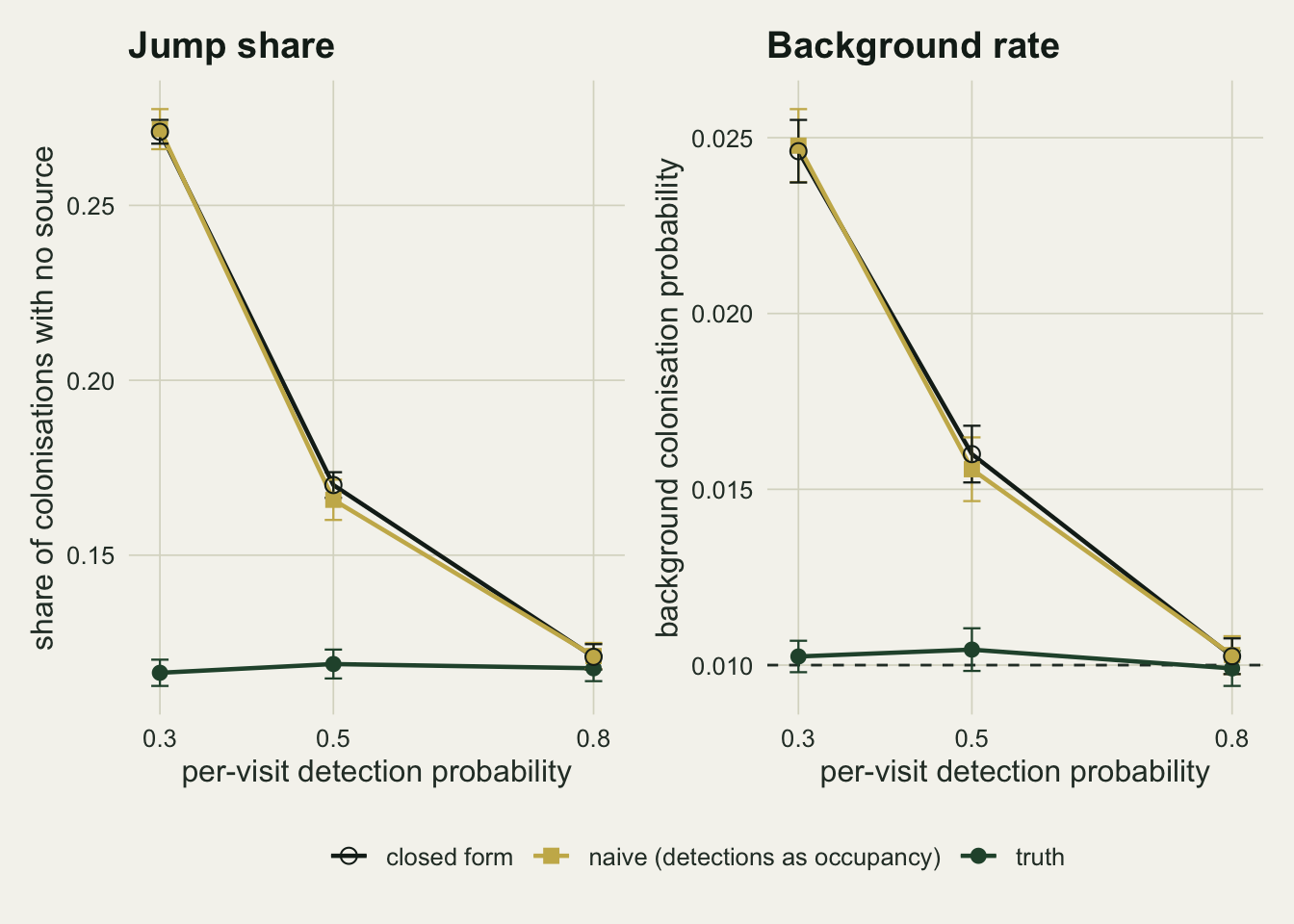
What the model recovers, and what the covariate costs it
The naive reading is not what a careful analyst would do. The obvious fix is the dynamic occupancy model, which knows about non-detection, with the observed neighbour count supplied as the covariate on colonisation. The oracle fit is the same model with the true neighbour count, and the difference between them is the price of the covariate, separated from everything else.
ml_over_or_low  <- avg$g0_ml[r_low] / avg$g0_or[r_low]
ml_over_or_mid  <- avg$g0_ml[r_mid] / avg$g0_or[r_mid]
ml_over_or_high <- avg$g0_ml[r_high] / avg$g0_or[r_high]
ml_over_true_low <- avg$g0_ml[r_low] / g0_true
or_over_true_low <- avg$g0_or[r_low] / g0_true
sm_over_true_low <- avg$g0_sm[r_low] / g0_true
sm_over_true_mid <- avg$g0_sm[r_mid] / g0_true
ml_over_true_mid <- avg$g0_ml[r_mid] / g0_true
sm_gap_low <- (avg$g0_sm[r_low] - g0_true) / sem$g0_sm[r_low]
excess_kept_low <- (ml_over_true_low - 1) / (g0_ratio_low - 1)
p_err_low  <- avg$p_ml[r_low] - p_grid[1]
eps_err_low <- avg$eps_ml[r_low] - eps_true
eps_err_or_low <- avg$eps_or[r_low] - eps_true
or_z_low <- abs((avg$g0_or[r_low] - g0_true) / sem$g0_or[r_low])
lift_z <- (ml_over_true_low - g0_ratio_mid) /
  sqrt((sem$g0_ml[r_low] / g0_true)^2 + (sem$g0_naive[r_mid] / g0_true)^2)
At a detection of 0.3 the fitted background rate with the observed covariate is 0.0177 and with the true covariate 0.0084, a ratio of 2.10. Against the design value of 0.01 the model with the observed covariate is 1.77 times high, so of the naive excess over the truth it has removed 48 per cent and kept 52 per cent. The oracle is not a neutral benchmark at this detection. It sits at 0.84 times the truth, 6.6 Monte Carlo standard errors below it, so 2.10 is a ratio to a depressed denominator. The 1.77 against the design value is the number to quote. Both halves are real: with poor detection this likelihood runs low on the background rate even when the covariate is perfect, and the observed covariate then pushes it high by more than that.
The price falls fast with detection. The ratio of the fitted background rate with the observed covariate to the oracle is 1.35 at a detection of 0.5 and 1.03 at 0.8. Put the other way round, the naive background rate at a detection of 0.5 is 1.56 times the truth, which is closer than the fitted model manages at a detection of 0.3 (1.77 times), by 3.5 Monte Carlo standard errors. For this parameter, lifting detection from three tenths to one half is worth more than fitting the model at three tenths. That is not the choice a programme actually faces, though: a programme surveying at one half would fit the model as well, and the two together land at 1.30 times the truth.
The smoothing pass overshoots at the low end. Refitting on the posterior expected neighbour count gives 0.0057 at a detection of 0.3, which is 0.57 times the truth and 19.0 Monte Carlo standard errors below it. The overshoot is not a tuning accident: an expected neighbour count is a smooth number between zero and four, so sites that truly had no occupied neighbour are given a fraction of one, the neighbour term is asked to explain colonisations that the background used to explain, and the background falls through the truth. At a detection of 0.5 it lands at 0.88 times the truth against 1.30 for the plug-in count, so it is the better of the two there but it is still low.
Detection and extinction are recovered less evenly than the headline suggests. With the observed covariate at a detection of 0.3 the fitted per-visit detection misses by -0.0136 and the extinction probability by -0.0252 against a truth of 0.10. The oracle misses extinction by +0.0173, in the other direction, so that parameter is absorbing part of the covariate error rather than tracking it. Nothing measured here identifies the route it takes.
g0_fit <- long_of(c("g0_ml", "g0_or", "g0_sm"),
                  c("observed neighbour count", "true count (oracle)",
                    "smoothed count"),
                  c("g0_ml", "g0_or", "g0_sm"))
gnb_fit <- long_of(c("gnb_ml", "gnb_or", "gnb_sm"),
                   c("observed neighbour count", "true count (oracle)",
                     "smoothed count"),
                   c("gnb_ml", "gnb_or", "gnb_sm"))
fit_cols <- c("observed neighbour count" = te_rust,
              "true count (oracle)" = te_forest, "smoothed count" = te_ink)
fit_shapes <- c("observed neighbour count" = 17,
                "true count (oracle)" = 16, "smoothed count" = 18)

panel_fit <- function(dat, y_lab, ttl, href) {
  ggplot(dat, aes(p, value, colour = series, shape = series)) +
    geom_hline(yintercept = href, linetype = "dashed", colour = te_body,
               linewidth = 0.5) +
    geom_line(linewidth = 0.8) +
    geom_errorbar(aes(ymin = value - 2 * se, ymax = value + 2 * se),
                  width = 0.02, linewidth = 0.4) +
    geom_point(size = 2.6) +
    scale_colour_manual(values = fit_cols, name = NULL) +
    scale_shape_manual(values = fit_shapes, name = NULL) +
    scale_x_continuous(breaks = p_grid) +
    labs(x = "per-visit detection probability", y = y_lab, title = ttl) +
    theme_datasheet() +
    theme(legend.position = "bottom")
}

(panel_fit(g0_fit, "background colonisation probability",
           "Background rate", g0_true) +
 panel_fit(gnb_fit, "per-neighbour colonisation probability",
           "Neighbour effect", gnb_true)) +
  plot_layout(guides = "collect") +
  plot_annotation(theme = theme_datasheet()) &
  theme(legend.position = "bottom")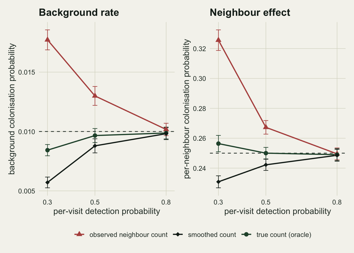
The neighbour effect goes up, not down
The right panel of that figure is the result that contradicts the reflex. Attenuation towards zero is what a mis-measured predictor does in a linear regression, and it is the direction the regression dilution post spends its length on. Here the per-neighbour colonisation probability moves the other way.
gnb_ratio_low  <- avg$gnb_ml[r_low] / gnb_true
gnb_or_low     <- avg$gnb_or[r_low] / gnb_true
gnb_ratio_high <- avg$gnb_ml[r_high] / gnb_true
gnb_d_low <- runs$gnb_ml[runs$p == p_grid[1]] - runs$gnb_or[runs$p == p_grid[1]]
gnb_z_low <- mean(gnb_d_low) / (sd(gnb_d_low) / sqrt(n_rep))
With the observed count at a detection of 0.3 the per-neighbour probability comes out at 0.326 against a truth of 0.25, a factor of 1.30. The oracle at the same detection gives 0.256, a factor of 1.03, and the two arms are 40 standard errors apart on the paired difference across the replicate grids. By a detection of 0.8 the observed-count fit is at 1.00 times the truth and the arms agree.
The reason the sign reverses is that the covariate is not measured with symmetric noise. A neighbour count built from detections can only be too low; it can never be too high, because a site that was never occupied cannot be detected. The count is censored downward, and the colonisations it has to explain are still there. The model responds by making each visible neighbour more potent, because visible neighbours are all it has. Classical regression dilution needs error that is independent of the truth; one-sided error that deletes signal from the predictor but not from the response pushes the coefficient up.
That matters for how the fit is read in a report. A per-neighbour effect that looks strong is not evidence that the covariate was well measured. Of the three product-form fits, the strongest neighbour effect and the worst background rate came from the same one.
The form error grows as the detection error shrinks
There are two ways to put the neighbour count into the colonisation probability, and they are not the same model. One is a logit-linear term, the reflex that comes with a link function: the log odds of colonisation linear in the number of occupied neighbours. The other is the product form used above, which says that each occupied neighbour gets its own independent attempt. Broms and colleagues write the colonisation probability in the second way; Bled and colleagues and Yackulic and colleagues model it as a function of latent or neighbourhood occupancy. To see what choosing the first costs, both are fitted with the true neighbour count, so that no covariate error is in play.
lg0_or_low  <- avg$lg0_or[r_low] / g0_true
lg0_or_mid  <- avg$lg0_or[r_mid] / g0_true
lg0_or_high <- avg$lg0_or[r_high] / g0_true
lg0_or_low_z <- (avg$lg0_or[r_low] - g0_true) / sem$lg0_or[r_low]
lg0_trend_z <- (avg$lg0_or[r_high] - avg$lg0_or[r_low]) /
  sqrt(sem$lg0_or[r_high]^2 + sem$lg0_or[r_low]^2)
form_vs_naive <- g0_ratio_low - lg0_or_high
lg4_or_high <- avg$lg4_or[r_high]
prod_or_high <- avg$g0_or[r_high] / g0_true
k_axis <- 0:4
curve_truth <- gam_true_k(k_axis)
curve_prod  <- 1 - (1 - avg$g0_or[r_high]) * (1 - avg$gnb_or[r_high])^k_axis
logit_slope <- qlogis(avg$lg1_or[r_high]) - qlogis(avg$lg0_or[r_high])
curve_logit <- plogis(qlogis(avg$lg0_or[r_high]) + logit_slope * k_axis)
form_curves <- data.frame(
  k = rep(k_axis, 3),
  value = c(curve_truth, curve_prod, curve_logit),
  series = rep(c("truth", "product form (true count)",
                 "logit-linear (true count)"), each = length(k_axis)))
cross_k <- k_axis[which(curve_logit > curve_truth & k_axis > 1)[1]]
At a detection of 0.8, where the survey sees almost everything, the logit-linear model fitted to the true neighbour count reports a background colonisation probability of 0.0227, which is 2.27 times the design value of 0.01. The product form on the same data and the same covariate reports 0.99 times the truth. The whole covariate problem at that level was worth a factor of 1.03; the form is worth 2.27. It is not the largest error in this post, though. The naive background rate at a detection of 0.3, read straight off detections with no model at all, was 2.48 times the truth, 0.21 higher again. What distinguishes the form is not the size of the error at one detection level but which way it moves across them.
The rest of the curve is not merely rescaled; it is bent. A line on the logit scale is convex in probability while it is low and concave once it is high, and the product form is concave over the whole range, so the two shapes cannot agree at more than a few points. With one occupied neighbour the logit-linear fit gives 0.134 against a truth of 0.258, with two 0.506 against 0.443, and with four 0.977 against 0.687. The fitted curve is high at no neighbours, low at one, and high again from 2 neighbours upward. Read as biology, that is a species that arrives from nowhere 2.3 times as often as it really does, underrates its first neighbour, and then saturates far too fast.
The bias is worse when detection is good, not better. At a detection of 0.3 the logit-linear background with the true count is 1.18 times the truth, at 0.5 1.84 times, and at 0.8 2.27 times, a trend of 17 standard errors end to end. The covariate error runs the other way over the same range, from 2.10 to 1.03. Part of what looks like a mild form bias at the low end is a cancellation: at that detection the correctly specified product form is itself pulled below the truth (the oracle lands at 0.84 times it), and that pull works against the form’s upward push. What survives it is still real, 4.3 standard errors above the truth. At 0.8 nothing pulls the estimate down and the form stands alone. Better fieldwork does not rescue a wrong functional form; it sharpens it.
ggplot(form_curves, aes(k, value, colour = series, shape = series)) +
  geom_line(linewidth = 0.9) +
  geom_point(size = 2.8) +
  scale_colour_manual(values = c("truth" = te_forest,
                                 "product form (true count)" = te_rust,
                                 "logit-linear (true count)" = te_gold),
                      name = NULL) +
  scale_shape_manual(values = c("truth" = 16,
                                "product form (true count)" = 17,
                                "logit-linear (true count)" = 15), name = NULL) +
  scale_x_continuous(breaks = 0:4) +
  labs(x = "occupied neighbours last season",
       y = "colonisation probability",
       title = "Two ways to write the same covariate",
       subtitle = "both fitted with the true neighbour count, detection 0.8") +
  theme_datasheet() +
  theme(legend.position = "bottom")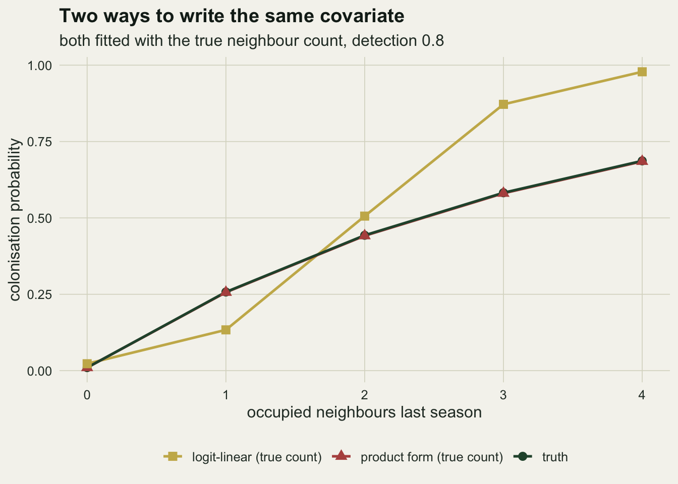
What to report
Never quote a jump share from raw detections. At a per-visit detection of 0.3 with 3 visits, the naive share of colonisations with no adjacent source was 2.34 times the truth in this experiment, and the naive background rate 2.48 times. Both errors are in the direction that argues for spending money on satellite hunting.
Report the season-level probability of missing an occupied site, not just the per-visit detection. That single number, q, is what drives the naive error, and it can be computed before the season starts: 0.3 per visit and 3 visits gives 0.343, while 0.8 per visit and the same three visits gives 0.008. Given the field of true occupancy, the average naive numbers follow from q alone, which is why the closed-form check above tracked the simulation mean to within 0.00043 on the background rate. One grid is looser: at a detection of 0.3 expect it to sit about 0.0021 away from the prediction.
Fit the neighbour term as a product, not as a logit-linear slope, unless there is a reason to prefer the second. On the true neighbour count at a detection of 0.8 the logit-linear form reported a background rate 2.27 times the truth where the product form reported 0.99 times, and it bent the response: 0.134 at one occupied neighbour against a truth of 0.258, and 0.977 at four against 0.687.
State which neighbour count went into the model. If it was the observed count, the background rate is biased upward and the per-neighbour effect upward as well, by 1.77 and 1.30 times the truth at a detection of 0.3 here. If the fit matters to a decision, run the latent-neighbour version. The one-pass smoothing repair used above is cheap and it removes the sign of the error, but at a detection of 0.3 it replaced an overestimate of 1.77 times the truth with an underestimate of 0.57 times, so it is a diagnostic rather than an answer.
Honest limits
The smoothing pass is not the model it stands in for. A latent-neighbour model puts the neighbour states in the likelihood and integrates over them; the pass here plugs a posterior mean into a covariate slot and refits once, which is a different estimator with no guarantee of consistency. Its over-correction at a detection of 0.3 is the visible symptom, and the full latent-state route, of the kind in Bayesian occupancy with latent-state MCMC, is what a decision-grade analysis needs. Nothing here tests whether a second or third smoothing pass converges to something sensible, and there is no reason to assume it does.
The truth in this experiment has exactly the product form that one of the fitted models assumes, so that model is correctly specified and the other is not. The comparison therefore measures the cost of departing from a known truth, not the cost of choosing between two forms when the truth is unknown. If real colonisation is logit-linear in neighbour count, the sign of that section reverses. What the section does establish is that the two forms are not interchangeable at the scale of the quantity being reported.
The grid is homogeneous. Every site has the same background rate, the same extinction probability and the same detection probability, and there is no habitat, no distance weighting beyond rook adjacency, and no variation in survey effort. Real neighbour counts are also spatially confounded with habitat, so a real fit would carry a habitat covariate that is itself correlated with the neighbour count, and the covariate error analysed here would be entangled with that collinearity.
Edge effects are ignored. Sites on the boundary of the grid have fewer than four neighbours, and the simulator treats the outside as permanently empty rather than wrapping the grid. That makes the boundary a sink for colonisation, which is realistic for a bounded study area but means the effective per-site neighbour count is slightly below four everywhere near the edge, for both the truth and the fits.
The jump definition is binary and adjacency-based, which is the coarsest possible version of the management question. A colonisation two cells from the nearest occupied site and one twenty cells away are both jumps here, and a real programme would care about the difference. A distance-weighted colonisation kernel would pose the same covariate-error problem in a form where the error also affects the estimated distance, which is not measured above.
Only 60 replicates were run per detection level, on a single grid size and a single set of process parameters. The ratios quoted are means over those replicates with their Monte Carlo standard errors attached, but nothing here maps the dependence of those ratios on the grid size, the number of seasons, or the size of the background rate relative to the neighbour effect. A background rate ten times larger would make the whole problem smaller, because the quantity being biased would no longer be near zero.
References
Bled F, Royle JA, Cam E 2011 Ecological Applications 21(1):290-302 (10.1890/09-1877.1)
Yackulic CB, Reid J, Davis R, Hines JE, Nichols JD, Forsman E 2012 Ecology 93(8):1953-1966 (10.1890/11-1709.1)
Broms KM, Hooten MB, Johnson DS, Altwegg R, Conquest LL 2016 Ecology 97(1):194-204 (10.1890/15-0416.1)
MacKenzie DI, Nichols JD, Hines JE, Knutson MG, Franklin AB 2003 Ecology 84(8):2200-2207 (10.1890/02-3090)