library(ggplot2)
library(dplyr)
library(tidyr)

ink <- "#16241d"; body <- "#2c3a31"; forest <- "#275139"; gold <- "#c9b458"
paper <- "#f5f4ee"; line_c <- "#dad9ca"; faint <- "#5d6b61"; sage <- "#93a87f"

theme_te <- function(base = 12) {
  theme_minimal(base_size = base) +
    theme(panel.grid.minor = element_blank(),
          panel.grid.major = element_line(colour = line_c, linewidth = 0.3),
          plot.background = element_rect(fill = paper, colour = NA),
          panel.background = element_rect(fill = paper, colour = NA),
          axis.title = element_text(colour = body),
          axis.text = element_text(colour = faint),
          plot.title = element_text(colour = ink, face = "bold"),
          plot.subtitle = element_text(colour = faint),
          legend.title = element_text(colour = body),
          legend.text = element_text(colour = faint))
}N-mixture models for abundance in R
R
abundance
detection
N-mixture
ecology tutorial
Estimate animal abundance from repeated counts while accounting for imperfect detection. Fit a binomial N-mixture model from scratch in R with base optim.
Count a species at a site on four separate visits and you rarely get the same number twice. Some individuals are present but missed on any given visit, so the raw counts sit below the true local abundance. If you take the mean count, or even the largest count seen, as your abundance figure, you are reporting detection times abundance rather than abundance itself.
The binomial N-mixture model of Royle (2004) separates these two quantities from nothing more than repeated counts. It treats the local abundance at each site as a latent Poisson variable and each visit as a binomial sample of the individuals that are there. Fitting it needs no marked animals and no distance measurements. This post builds the likelihood by hand with optim, so the machinery is fully visible, and then checks whether the fitted model actually reproduces the count data.
The model
Let there be R sites, each visited K times. Write the latent abundance at site i as a Poisson variable with mean lambda, and let each present individual be counted on a visit with probability p. The count on visit k at site i is then binomial:
\[N_i \sim \text{Poisson}(\lambda), \qquad y_{ik} \mid N_i \sim \text{Binomial}(N_i, p).\]
We never observe N_i. The likelihood for a site integrates it out by summing over every abundance that could have produced the counts, from the largest count seen up to a safe upper bound:
\[P(y_{i1}, \dots, y_{iK}) = \sum_{N = \max_k y_{ik}}^{\infty} \text{Poisson}(N; \lambda) \prod_{k=1}^{K} \text{Binomial}(y_{ik}; N, p).\]
The repeated visits are what make lambda and p separable: a site that reads 0, 3, 1, 2 across visits cannot have a very low abundance with high detection, nor a very high abundance with tiny detection, and the spread across visits pins both down.
Simulating a survey
We generate 150 sites with four visits each, a mean abundance of 2.6 individuals, and a per-visit detection probability of 0.35. Setting the seed immediately before the draws keeps the numbers reproducible.
set.seed(2027)
R <- 150            # sites
K <- 4              # repeat visits
lambda_true <- 2.6  # mean local abundance
p_true <- 0.35      # per-visit detection probability

N <- rpois(R, lambda_true)                       # latent abundance, never observed
y <- matrix(NA_integer_, R, K)
for (k in 1:K) y[, k] <- rbinom(R, N, p_true)    # binomial counts given N

head(y)
[,1] [,2] [,3] [,4]
[1,] 0 1 0 0
[2,] 1 1 1 0
[3,] 0 0 1 1
[4,] 0 1 2 1
[5,] 0 2 1 1
[6,] 0 1 0 0What the naive counts tell you
Before fitting anything, look at the two summaries a field report might quote: the mean count per visit and the largest count seen at each site. Both fall well short of the simulation truth.
maxcount <- apply(y, 1, max)
meancount <- rowMeans(y)

c(true_mean_N = mean(N),
  naive_mean_of_max = mean(maxcount),
  naive_mean_of_mean = mean(meancount))
true_mean_N naive_mean_of_max naive_mean_of_mean
2.8000000 1.6400000 0.9366667 c(true_total_N = sum(N), naive_total_from_max = sum(maxcount)) true_total_N naive_total_from_max
420 246 The mean of the per-site maxima is about 1.64, against a true mean abundance of 2.8 in this sample. Summed across sites the maximum-count total is 246 individuals where 420 are actually present. The mean count fares worse still, because it averages in the visits that missed animals. Neither summary is wrong as a description of what was counted; both are simply the wrong quantity if you want abundance.
Fitting the model by hand
The negative log-likelihood loops over sites and, for each, sums the joint Poisson and binomial probability over candidate abundances. We work on the log scale for lambda and the logit scale for p so the optimiser is unconstrained, then read the estimates back on their natural scales.
Nmax <- 60   # upper bound for the sum; well above any plausible abundance here

negll <- function(par) {
  lam <- exp(par[1])
  p   <- plogis(par[2])
  ll  <- 0
  for (i in 1:R) {
    lo <- max(y[i, ])          # abundance cannot be below the largest count seen
    Ns <- lo:Nmax
    pmfN <- dpois(Ns, lam)
    lik_i <- 0
    for (j in seq_along(Ns)) {
      lik_i <- lik_i + pmfN[j] * prod(dbinom(y[i, ], Ns[j], p))
    }
    ll <- ll + log(lik_i)
  }
  -ll
}

fit <- optim(c(log(2), qlogis(0.3)), negll, method = "BFGS", hessian = TRUE)
lam_hat <- exp(fit$par[1])
p_hat   <- plogis(fit$par[2])
c(lambda_hat = lam_hat, p_hat = p_hat)
lambda_hat p_hat
2.5216550 0.3714492 Standard errors come from the Hessian on the estimation scale. Because the parameters were transformed, the delta method carries the standard errors back to the natural scales, and the confidence intervals are built on the estimation scale and then transformed so they stay inside the valid range.
se_link <- sqrt(diag(solve(fit$hessian)))
se_lam <- se_link[1] * lam_hat               # derivative of exp is exp
se_p   <- se_link[2] * p_hat * (1 - p_hat)   # derivative of plogis
lam_ci <- exp(fit$par[1] + c(-1.96, 1.96) * se_link[1])
p_ci   <- plogis(fit$par[2] + c(-1.96, 1.96) * se_link[2])

round(c(lambda_hat = lam_hat, se = se_lam, lo = lam_ci[1], hi = lam_ci[2]), 3)
lambda_hat se lo hi
2.522 0.264 2.054 3.096 round(c(p_hat = p_hat, se = se_p, lo = p_ci[1], hi = p_ci[2]), 3)p_hat se lo hi
0.371 0.036 0.304 0.444 The estimate of lambda is about 2.52 with a 95% interval of roughly 2.05 to 3.10, comfortably covering the true 2.6. Detection comes out at 0.37, close to the true 0.35, meaning a single visit misses around three individuals in five. Multiplying the two gives 0.94, which matches the observed grand mean count exactly: the model has split that product into its abundance and detection parts.
d1 <- data.frame(
  est = factor(c("Naive: mean\nmax count", "N-mixture\nlambda-hat", "Truth\n(lambda)"),
               levels = c("Naive: mean\nmax count", "N-mixture\nlambda-hat", "Truth\n(lambda)")),
  val = c(mean(maxcount), lam_hat, lambda_true),
  lo  = c(NA, lam_ci[1], NA),
  hi  = c(NA, lam_ci[2], NA),
  fill = c("naive", "model", "truth"))

ggplot(d1, aes(est, val, fill = fill)) +
  geom_col(width = 0.62) +
  geom_errorbar(aes(ymin = lo, ymax = hi), width = 0.16, colour = ink, na.rm = TRUE) +
  geom_hline(yintercept = lambda_true, linetype = "dashed", colour = faint, linewidth = 0.4) +
  scale_fill_manual(values = c(naive = gold, model = forest, truth = sage), guide = "none") +
  labs(title = "Ignoring detection undercounts abundance",
       subtitle = "Mean local abundance: naive max count versus the N-mixture estimate",
       x = NULL, y = "Individuals per site") +
  theme_te()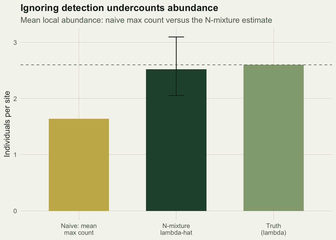
Does the fitted model fit the data?
An estimate you cannot check is worth little, and N-mixture models are known to give confident but wrong answers when their assumptions fail. A first, cheap check is whether the fitted model reproduces the distribution of counts. Under the model the chance of seeing a count of c on a visit is again a Poisson and binomial sum, and we can compare that to the observed frequencies.
cmax <- max(y)
cs <- 0:cmax
obs <- as.numeric(table(factor(as.vector(y), levels = cs))) / (R * K)
expf <- sapply(cs, function(c) {
  Ns <- c:Nmax
  sum(dpois(Ns, lam_hat) * dbinom(c, Ns, p_hat))
})

d2 <- data.frame(count = rep(cs, 2),
                 freq = c(obs, expf),
                 src = rep(c("Observed", "Fitted N-mixture"), each = length(cs)))
d2$src <- factor(d2$src, levels = c("Observed", "Fitted N-mixture"))

ggplot(d2, aes(factor(count), freq, fill = src)) +
  geom_col(position = position_dodge(width = 0.7), width = 0.62) +
  scale_fill_manual(values = c("Observed" = sage, "Fitted N-mixture" = forest), name = NULL) +
  labs(title = "The fitted model reproduces the count distribution",
       subtitle = "Relative frequency of per-visit counts, pooled over sites and visits",
       x = "Count on a visit", y = "Relative frequency") +
  theme_te() +
  theme(legend.position = c(0.8, 0.8))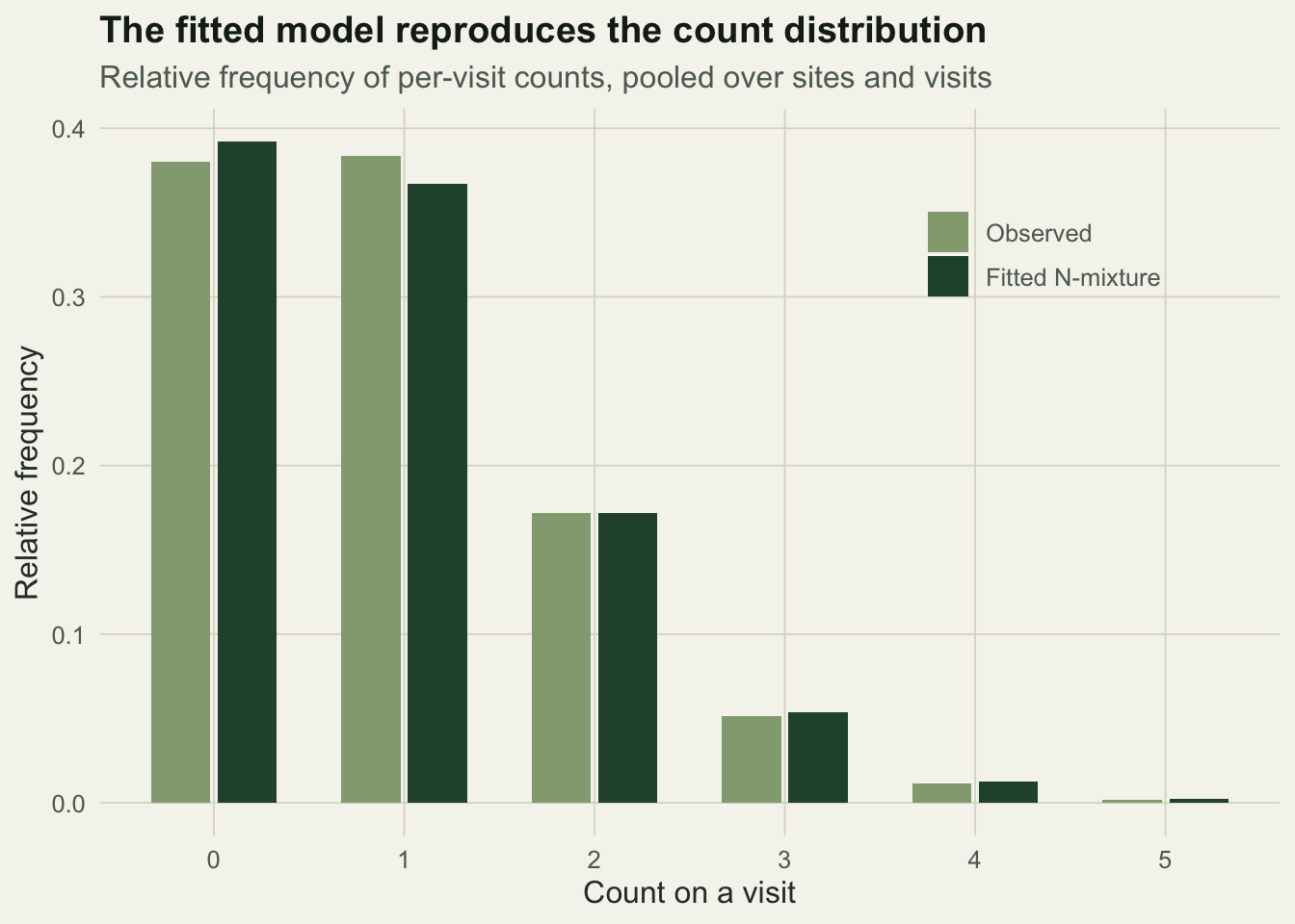
The observed and expected bars track each other at every count, which is reassuring here because the data were generated from exactly this model. On real data a mismatch, especially an excess of high counts, is the usual sign that abundance varies more than a Poisson allows or that detection is not constant.
Abundance at each site
The same integration that gives the likelihood also gives a posterior mean abundance for each site: weight every candidate abundance by how well it explains that site’s counts. Plotting these against the raw maximum shows the correction the model applies.
postN <- numeric(R)
for (i in 1:R) {
  lo <- max(y[i, ]); Ns <- lo:Nmax
  w <- dpois(Ns, lam_hat) * sapply(Ns, function(Nj) prod(dbinom(y[i, ], Nj, p_hat)))
  postN[i] <- sum(Ns * w) / sum(w)
}
c(estimated_total = sum(postN), naive_max_total = sum(maxcount), true_total = sum(N))
estimated_total naive_max_total true_total
378.2483 246.0000 420.0000 d3 <- data.frame(maxc = maxcount, post = postN)
ggplot(d3, aes(maxc, post)) +
geom_abline(slope = 1, intercept = 0, linetype = "dashed", colour = faint) +
geom_point(position = position_jitter(width = 0.12, height = 0, seed = 7),
colour = forest, alpha = 0.5, size = 1.9) +
labs(title = "Site abundance is corrected upward from the raw maximum",
subtitle = "Posterior-mean local abundance versus the largest count seen at a site",
x = "Observed maximum count", y = "Estimated abundance (posterior mean)") +
theme_te()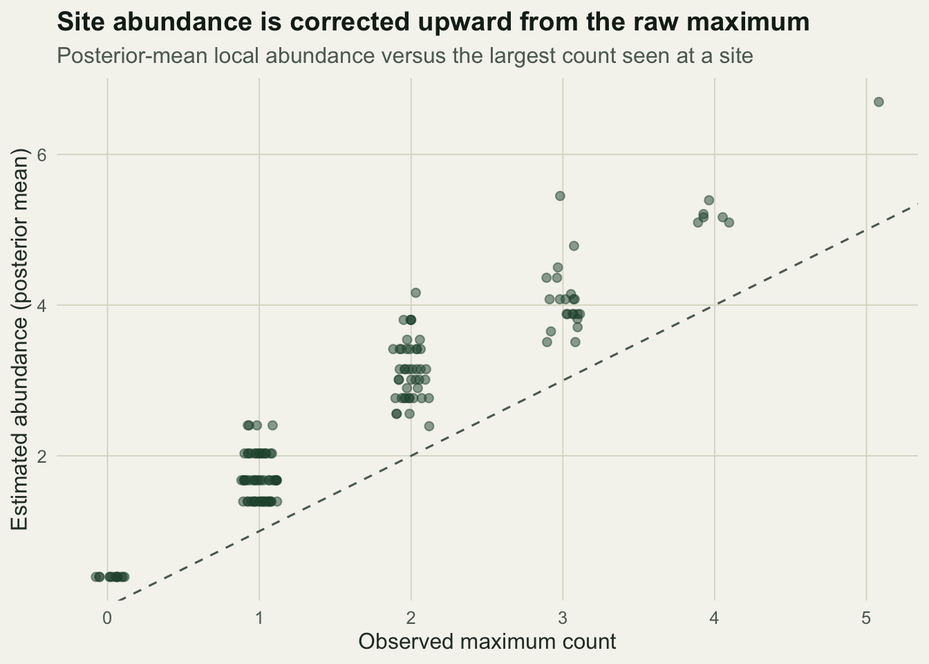
Every point sits above the identity line, because the model recognises that even the best visit at a site probably missed someone. Summed over sites the estimated total is about 378 individuals, against 246 from the raw maxima and a true total of 420. The estimate still sits a little below the truth in this particular sample, which is the honest reality of estimating a latent quantity from sparse counts.
When not to trust the estimate
N-mixture models buy abundance without marking animals, and that bargain has limits. Barker and colleagues (2018) show, from a capture-recapture viewpoint, that the information lost by not identifying individuals is real, and that plausible alternative models can fit the same counts while implying very different abundances. Uncontrolled variation in detection is especially damaging, since the model can trade it against abundance. Kery (2018) screened 137 bird data sets and found Poisson mixtures usually identifiable, but negative-binomial mixtures unidentifiable in a quarter of cases despite often being favoured by AIC.
The practical advice that follows is plain: check that the model is identifiable, compare the fitted count distribution to the data as above, be wary of a negative-binomial mixture chosen purely on AIC, and treat the abundance figure as conditional on the closure and constant-detection assumptions holding over the survey. Where marking is feasible, a capture-recapture design carries more information per unit effort.
References
Royle 2004 Biometrics 60(1):108-115 (10.1111/j.0006-341X.2004.00142.x)
Barker, Schofield, Link and Sauer 2018 Biometrics 74(1):369-377 (10.1111/biom.12734)
Kery 2018 Ecology 99(2):281-288 (10.1002/ecy.2093)
Kery and Royle 2016 Applied Hierarchical Modeling in Ecology, Volume 1 (Academic Press, ISBN 978-0-12-801378-6)