---
title: "Metropolis-Hastings from scratch"
description: "Code a random-walk Metropolis sampler by hand in R to estimate a survival probability, and see why the posterior beats a Wald interval that dips below zero."
date: "2026-07-14 09:00"
categories: [Bayesian statistics, MCMC, R, survival, ecology tutorial]
image: thumbnail.png
image-alt: "Posterior density for a survival probability with the exact Beta curve and a symmetric Wald approximation that extends below zero."
---
Almost every quantity an ecologist reports is really a small number pulled from a noisy sample: a survival probability from a handful of tagged animals, a prevalence from a few positive tests, a detection rate from a short survey. The usual point estimate plus a plus-or-minus interval works well when the sample is large and the estimate sits comfortably away from a boundary. When it does not, the standard interval can wander into impossible territory. This post builds the workhorse of Bayesian computation, the Metropolis-Hastings sampler, in a few lines of base R, and uses it to get a survival probability that respects the boundary. Because the example is deliberately simple, we can also check the sampler against an answer we know exactly.
```{r}
#| label: setup
#| include: false
library(ggplot2)
knitr::opts_chunk$set(echo = TRUE, message = FALSE, warning = FALSE,
fig.align = "center", dpi = 150)
paper <- "#f5f4ee"; ink <- "#16241d"; forest <- "#275139"; sage <- "#93a87f"
line_col <- "#dad9ca"; faint <- "#5d6b61"; accent2 <- "#c9b458"; warm <- "#cda23f"; brick <- "#b5534e"
theme_te <- function(base = 12) theme_minimal(base_size = base) + theme(
plot.background = element_rect(fill = paper, colour = NA),
panel.background = element_rect(fill = paper, colour = NA),
panel.grid.major = element_line(colour = line_col, linewidth = 0.3),
panel.grid.minor = element_blank(),
axis.title = element_text(colour = ink), axis.text = element_text(colour = faint),
plot.title = element_text(colour = ink, face = "bold"),
plot.subtitle = element_text(colour = faint),
legend.title = element_text(colour = ink), legend.text = element_text(colour = faint),
legend.position = "top",
strip.text = element_text(colour = ink, face = "bold"))
theme_set(theme_te())
```
## A small sample and a naive interval
Twenty juveniles are radio-tagged at fledging; two are still alive at the first-year census. We want the first-year survival probability. The obvious estimate is the observed fraction, and the textbook interval is the Wald (normal) approximation on that fraction.
```{r}
#| label: data-wald
n <- 20L; y <- 2L
p_hat <- y / n
wald_se <- sqrt(p_hat * (1 - p_hat) / n)
wald_ci <- p_hat + c(-1, 1) * 1.96 * wald_se
round(c(estimate = p_hat, se = wald_se, lower = wald_ci[1], upper = wald_ci[2]), 4)
```
The point estimate is `r round(p_hat, 2)`, and the Wald interval runs from `r round(wald_ci[1], 3)` to `r round(wald_ci[2], 3)`. The lower limit is below zero, which is nonsense for a probability. The Wald interval is symmetric by construction, and near a boundary that symmetry is exactly wrong: it pushes mass into a region where the parameter cannot live. About `r round(pnorm(0, p_hat, wald_se) * 100, 1)` per cent of the implied normal sits below zero. We want an interval that knows a probability lives in the unit range and that leans the way the data lean.
## A Bayesian model with a known answer
Put a prior on the survival probability and combine it with the likelihood. With `y` survivors out of `n` and a Beta prior, the posterior is another Beta, because the Beta and the binomial are conjugate. A flat Beta(1, 1) prior gives a posterior of Beta(1 + `y`, 1 + `n` - `y`).
```{r}
#| label: exact-posterior
a0 <- 1; b0 <- 1                       # Beta(1, 1) prior: flat on (0, 1)
a_post <- a0 + y
b_post <- b0 + (n - y)                  # exact posterior: Beta(a_post, b_post)
exact <- c(mean   = a_post / (a_post + b_post),
           median = qbeta(0.5,   a_post, b_post),
           lower  = qbeta(0.025, a_post, b_post),
           upper  = qbeta(0.975, a_post, b_post))
round(exact, 4)
```
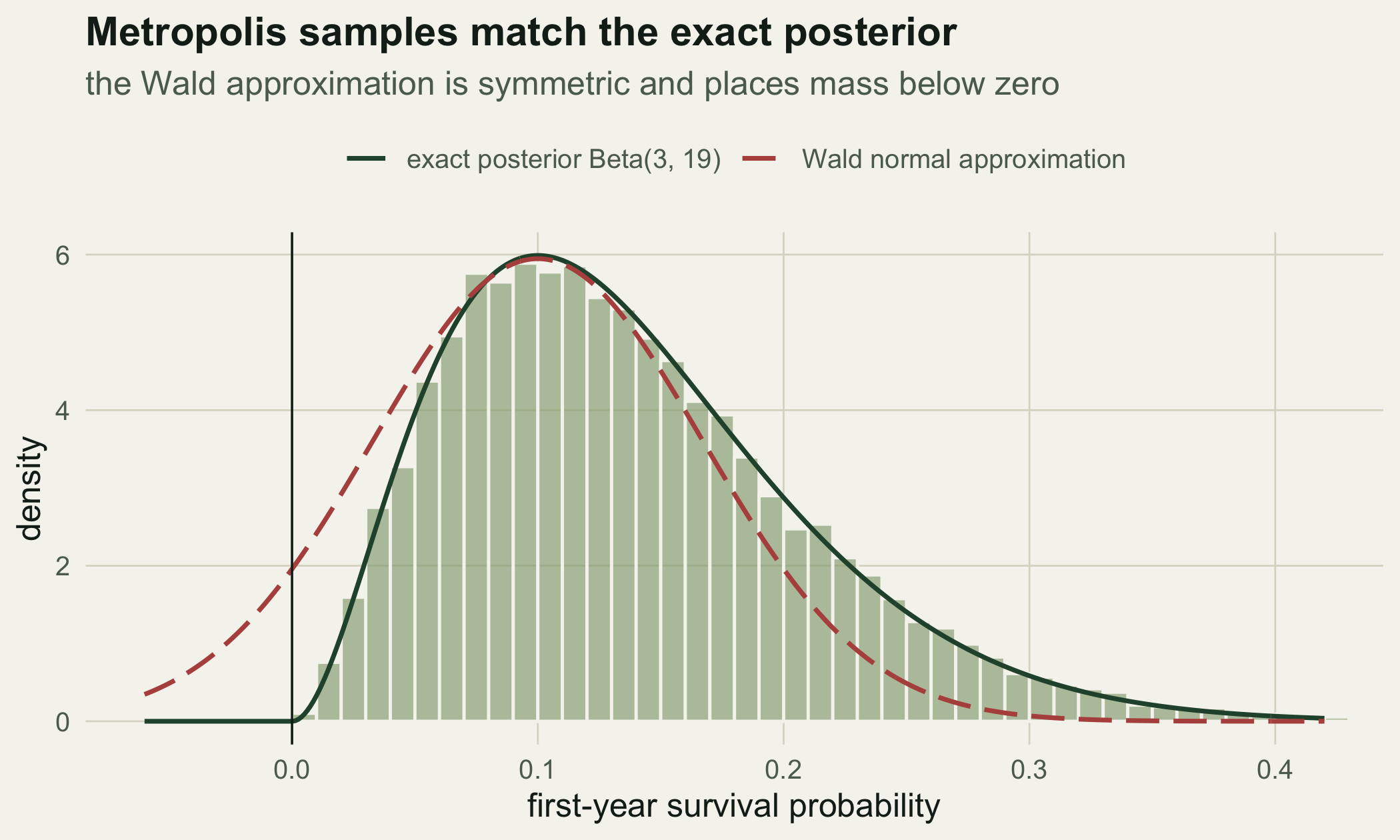
The exact posterior is Beta(`r a_post`, `r b_post`), with mean `r round(exact["mean"], 3)`, median `r round(exact["median"], 3)`, and a 95 per cent credible interval of `r round(exact["lower"], 3)` to `r round(exact["upper"], 3)`. It sits inside the unit range, it is skewed to the right, and its lower limit is a sensible `r round(exact["lower"], 3)` rather than a negative number. Conjugacy hands us this in closed form, which makes it the ideal target for checking a sampler: if the Metropolis machine cannot reproduce a Beta, it is broken.
## Random-walk Metropolis, by hand
Most real models are not conjugate, so we cannot read the posterior off a table. Metropolis-Hastings sidesteps that. It walks around the parameter space, and at each step it proposes a small move and either accepts it or stays put. The accept rule uses only the ratio of the posterior at the proposed and current values, so the awkward normalising constant of the posterior cancels and never has to be computed.
The recipe for a symmetric random-walk proposal is short. Propose a candidate by adding Gaussian noise to the current value. Compute the log posterior at both points (here the log prior plus the log likelihood). Accept the candidate with probability equal to the exponential of the log-posterior difference, capped at one; otherwise keep the current value. Record the value either way.
```{r}
#| label: sampler
log_post <- function(theta) {
  if (theta <= 0 || theta >= 1) return(-Inf)          # zero prior outside (0, 1)
  dbeta(theta, a0, b0, log = TRUE) + dbinom(y, n, theta, log = TRUE)
}

metropolis <- function(n_iter, prop_sd, init = 0.5) {
  draws <- numeric(n_iter)
  acc <- 0L
  cur <- init
  cur_lp <- log_post(cur)
  for (i in seq_len(n_iter)) {
    prop    <- cur + rnorm(1, 0, prop_sd)             # symmetric random-walk step
    prop_lp <- log_post(prop)
    if (log(runif(1)) < prop_lp - cur_lp) {           # accept on the log scale
      cur <- prop; cur_lp <- prop_lp; acc <- acc + 1L
    }
    draws[i] <- cur                                   # record accepted or repeated value
  }
  list(draws = draws, acc_rate = acc / n_iter)
}
```
A candidate outside the unit range gets a log posterior of minus infinity and is rejected automatically, so the sampler stays where a probability is allowed to live. That is all Metropolis is: propose, compare, keep or discard.
## Tuning the proposal width
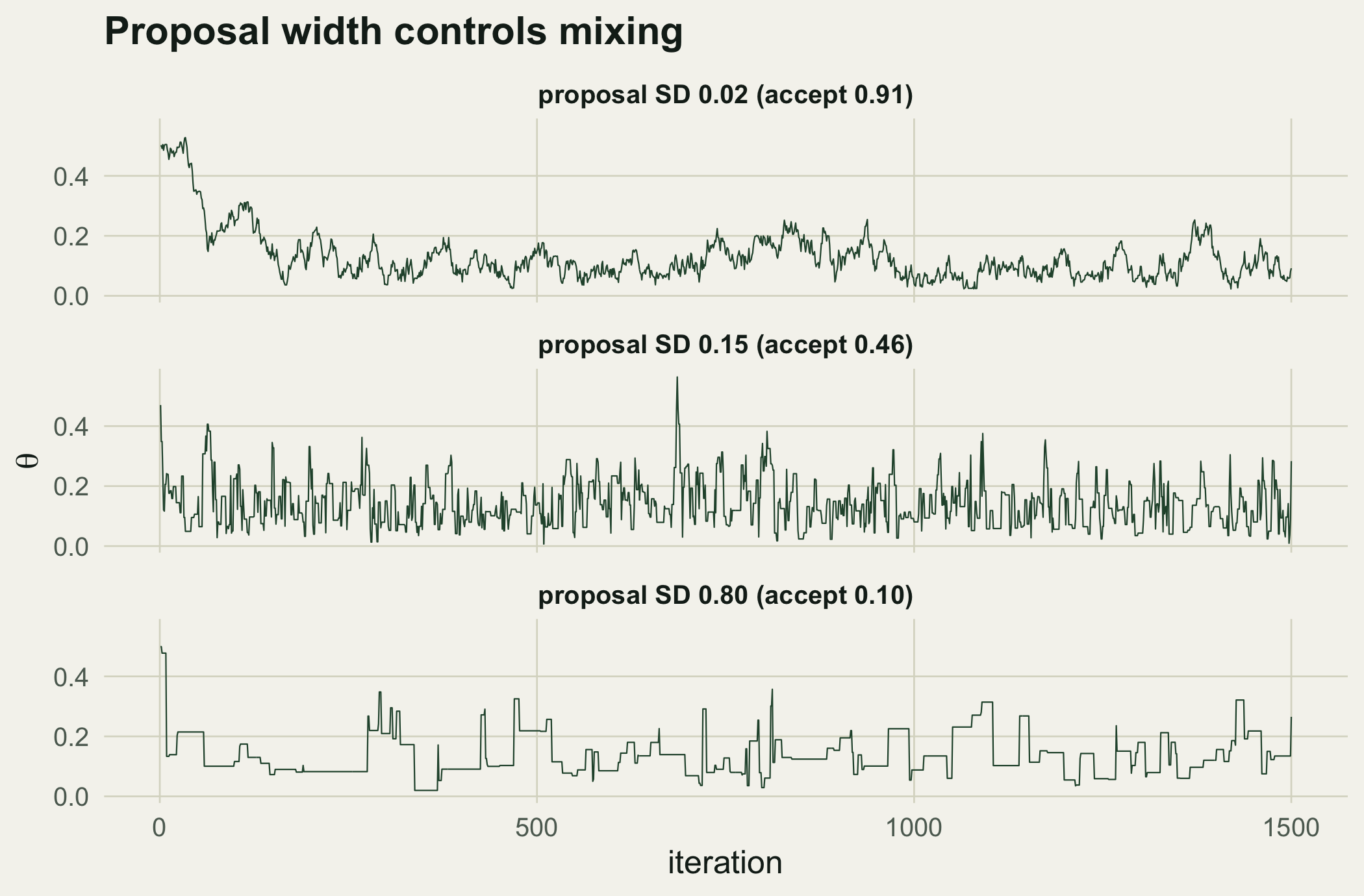
The one dial is the proposal standard deviation. Too small and every step is accepted but the walk crawls, so successive draws are nearly identical. Too large and almost every step lands in a low-density region and is rejected, so the chain sticks in place for long stretches. Both explore the posterior slowly. The sweet spot for a one-dimensional target accepts a little under half of its proposals.
```{r}
#| label: run-chains
n_iter <- 40000L; burn <- 2000L
set.seed(4914)
small <- metropolis(n_iter, prop_sd = 0.02)
good  <- metropolis(n_iter, prop_sd = 0.15)
large <- metropolis(n_iter, prop_sd = 0.80)
round(c(small = small$acc_rate, good = good$acc_rate, large = large$acc_rate), 3)
```
The narrow proposal accepts `r round(small$acc_rate * 100)` per cent of moves, the wide one only `r round(large$acc_rate * 100)` per cent, and the middle one `r round(good$acc_rate * 100)` per cent. The traces below tell the same story visually. The narrow chain drifts in smooth, slow sweeps; the wide chain shows flat plateaus where it kept rejecting; the middle chain fills the posterior with a healthy fuzz.
```{r}
#| label: fig-traces
#| fig-cap: "Trace of the first 1500 iterations for three proposal widths. A narrow proposal accepts almost everything but drifts slowly; a wide proposal rejects almost everything and sticks; the middle width mixes well."
#| fig-alt: "Three stacked trace plots of the survival probability against iteration. The top panel drifts slowly, the middle panel fills the range evenly, and the bottom panel shows long flat stretches."
#| fig-width: 7
#| fig-height: 4.6
K <- 1500
mk <- function(ch, lab) data.frame(iter = 1:K, theta = ch$draws[1:K],
        chain = sprintf("%s (accept %.2f)", lab, ch$acc_rate))
tr <- rbind(mk(small, "proposal SD 0.02"), mk(good, "proposal SD 0.15"), mk(large, "proposal SD 0.80"))
tr$chain <- factor(tr$chain, levels = unique(tr$chain))
ggplot(tr, aes(iter, theta)) +
  geom_line(colour = forest, linewidth = 0.25) +
  facet_wrap(~chain, ncol = 1) +
  labs(x = "iteration", y = expression(theta), title = "Proposal width controls mixing")
```
Acceptance rate is a rough tuning guide, not a quality certificate. The narrow chain here accepts nearly everything yet mixes worst; a companion post on convergence diagnostics shows how to measure mixing directly rather than eyeballing a trace.
## Reading off the posterior
Drop the first `r burn` iterations as burn-in and summarise the rest of the well-tuned chain. Any posterior quantity is just a summary of the stored draws: the mean, the median, quantiles for a credible interval, or the fraction of draws above a threshold you care about.
```{r}
#| label: posterior-summary
g  <- good$draws[(burn + 1):n_iter]
mh <- c(mean   = mean(g),
        median = median(g),
        lower  = unname(quantile(g, 0.025)),
        upper  = unname(quantile(g, 0.975)))
round(mh, 4)
```
The sampled posterior mean is `r round(mh["mean"], 3)` against the exact `r round(exact["mean"], 3)`, and the 95 per cent credible interval of `r round(mh["lower"], 3)` to `r round(mh["upper"], 3)` sits on top of the exact `r round(exact["lower"], 3)` to `r round(exact["upper"], 3)`. The sampler reproduces the Beta it never knew it was targeting, to within a whisker of Monte Carlo error. The figure overlays the draws, the exact curve, and the Wald normal on one axis.
```{r}
#| label: fig-posterior
#| fig-cap: "Metropolis draws (bars), the exact Beta(3, 19) posterior (solid), and the Wald normal approximation (dashed). The samples trace the exact posterior; the Wald curve is symmetric and spills below zero."
#| fig-alt: "A histogram of posterior draws with a solid forest curve tracing it closely and a dashed red normal curve that is shifted left and extends past the vertical line at zero."
#| fig-width: 7
#| fig-height: 4.2
xs <- seq(-0.06, 0.42, length.out = 400)
curv <- rbind(
  data.frame(x = xs, dens = dbeta(pmin(pmax(xs, 1e-9), 1 - 1e-9), a_post, b_post) * (xs > 0 & xs < 1),
             src = "exact posterior Beta(3, 19)"),
  data.frame(x = xs, dens = dnorm(xs, p_hat, wald_se), src = "Wald normal approximation"))
curv$src <- factor(curv$src, levels = c("exact posterior Beta(3, 19)", "Wald normal approximation"))
ggplot() +
  geom_histogram(data = data.frame(g = g), aes(g, after_stat(density)),
                 binwidth = 0.01, boundary = 0, fill = sage, colour = paper, alpha = 0.65) +
  geom_line(data = curv, aes(x, dens, colour = src, linetype = src), linewidth = 0.8) +
  geom_vline(xintercept = 0, colour = ink, linewidth = 0.4) +
  scale_colour_manual(values = c(forest, brick), name = NULL) +
  scale_linetype_manual(values = c("solid", "longdash"), name = NULL) +
  coord_cartesian(xlim = c(-0.06, 0.42)) +
  labs(x = "first-year survival probability", y = "density",
       title = "Metropolis samples match the exact posterior",
       subtitle = "the Wald approximation is symmetric and places mass below zero")
```
## What the sampler buys you
The payoff is not a better point estimate; both methods land near a tenth. The payoff is an honest description of the whole uncertainty. The posterior stays inside the unit range, its skew shows that a survival much higher than the point estimate is more plausible than a much lower one, and any downstream quantity follows for free. If a management rule triggers when first-year survival exceeds a quarter, the posterior answers directly: about `r round(mean(g > 0.25) * 100)` per cent of the draws clear that mark. There is no delta-method calculation and no worry about a normal approximation failing at the edge.
For a conjugate one-parameter model you would never actually need Metropolis, and that is the point of using one here: the closed form lets us confirm the sampler is correct before we point it at models with no closed form. From here, two directions open up. When every full conditional is itself a standard distribution, Gibbs sampling avoids tuning altogether. And whatever the sampler, a single well-behaved trace is not proof of convergence; that needs several chains and a numerical check.
## Related tutorials
- [Gibbs sampling with conjugate updates](../gibbs-sampling-conjugate/)
- [MCMC convergence diagnostics from scratch](../mcmc-convergence-diagnostics/)
- [Standard errors and confidence intervals](../standard-errors-confidence-intervals/)
- [Bootstrap confidence intervals](../bootstrap-confidence-intervals/)
## References
- Metropolis N, Rosenbluth AW, Rosenbluth MN, Teller AH, Teller E 1953 Journal of Chemical Physics 21(6):1087-1092 (10.1063/1.1699114)
- Hastings WK 1970 Biometrika 57(1):97-109 (10.1093/biomet/57.1.97)
- Roberts GO, Gelman A, Gilks WR 1997 Annals of Applied Probability 7(1):110-120 (10.1214/aoap/1034625254)
- Ellison AM 2004 Ecology Letters 7(6):509-520 (10.1111/j.1461-0248.2004.00603.x)
- Gelman A, Carlin JB, Stern HS, Dunson DB, Vehtari A, Rubin DB 2013 Bayesian Data Analysis, 3rd edition (ISBN 978-1-4398-4095-5)
- McCarthy MA 2007 Bayesian Methods for Ecology (ISBN 978-0-521-85057-5)