Familiarity covariates without memory

A familiarity covariate built from an animal’s own past fixes can absorb a layer or home range left out of a step selection model. Measured in R, with placebos.

A wild boar wears a GPS collar for a season, and the analyst fitting a step selection function to its fixes wants to know whether it returns to places it knows. The usual way to ask is to build a familiarity layer from the animal’s own track, a kernel density of where it has been before, recomputed at every step, and to put that layer into the model next to the habitat covariates. Oliveira-Santos and colleagues (2016) did this for feral hogs, with dynamic maps of past residence time as a surrogate for memory, and found the hogs choosing previously visited places; the ways animals use spatial memory are reviewed by Fagan and colleagues (2013). The coefficient on familiarity comes out positive and significant, and it reads as memory.

The trouble is that familiarity is built from the track, and the track goes wherever the animal likes to be, for whatever reason. A habitat layer that is not in the model, or a home range that keeps pulling the animal back, puts fixes in the same places again and again, and a kernel density of past fixes is high exactly there. The familiarity term can carry that omitted structure, and nothing in the fitted model says which of the two it is carrying. The temporal version of the trap is measured in Self-exciting events and the Hawkes process, in its section on a slow background: a Hawkes model with a constant background rate reports strong self-excitation in detections that have none, because the only way it can put more events into a good day is to let each event call up the next. This post carries that principle from time into space. The familiarity term plays the part of the excitation kernel; the missing layer and the home range play the part of the slow background. The same post names a second lever that time offers, direction: provoked events follow earlier events and never precede them, a lever it says it does not isolate. The future-fix placebo tried below is that lever carried into space, and on its own it turns out to be of no use.

The step selection machinery is the conditional logistic likelihood of Fortin and colleagues (2005), as built in Step selection functions for animal movement, with the step length terms of Avgar and colleagues (2016) from Integrated step selection analysis in R. Every habitat covariate in those posts is a fixed map; none is computed from the animal’s own history. Validating a step selection model shows a significant coefficient that tells the wrong story because a covariate has the wrong shape. Here the covariate has a reasonable shape and the wrong content. Levy walk or patchy habitat is a relative from the other side of movement ecology: there a pattern read as a rule of the animal, a power-law search, is produced by the habitat it walks through.

Two simulated animals carry the argument, one that never remembers anything and one that selects on its own past familiarity. Both are fitted with the familiarity term, first with a layer and the home range left out and then with both put back. Along the way the post tries the checks an analyst would reach for: a placebo layer built from where the animal goes later, which no memory can use; the past and the future layers in one model; and a flexible surface in the coordinates standing in for structure the analyst cannot name.

library(survival)
library(ggplot2)

te_paper  <- "#f5f4ee"
te_ink    <- "#16241d"
te_body   <- "#2c3a31"
te_forest <- "#275139"
te_rust   <- "#b5534e"
te_gold   <- "#c9b458"
te_line   <- "#dad9ca"

theme_datasheet <- function() {
  theme_minimal(base_size = 12) +
    theme(plot.background  = element_rect(fill = te_paper, colour = NA),
          panel.background = element_rect(fill = te_paper, colour = NA),
          panel.grid.major = element_line(colour = te_line, linewidth = 0.3),
          panel.grid.minor = element_blank(),
          text             = element_text(colour = te_body),
          plot.title       = element_text(colour = te_ink, face = "bold"),
          plot.subtitle    = element_text(colour = te_body),
          axis.text        = element_text(colour = te_body),
          strip.text       = element_text(colour = te_ink, face = "bold"))
}

Two layers, a home range and two animals

The landscape has two habitat layers made of sine waves. Layer A, sin(x / 7) + cos(y / 9), is the one the analyst has. Layer B, 0.8 * sin((x - y) / 6), is a second layer the animal selects just as strongly and the analyst does not have, a forage map nobody made. A home range enters as a pull towards the origin, minus 0.002 times the squared distance from it, which keeps each track bounded. At every step the animal draws 30 candidate moves from a gamma step length with shape 2 and scale 1.5 and a uniform direction, and takes one of them with probability proportional to exp(A + B - 0.002 r^2) at its end. The choice uses the Gumbel-max trick, which draws from exactly those probabilities and vectorises over tracks.

layer_a  <- function(x, y) sin(x / 7) + cos(y / 9)
layer_b  <- function(x, y) 0.8 * sin((x - y) / 6)
pull     <- 0.002       # range attraction: minus pull times squared distance from home
gam_mem  <- 0.5         # selection on past familiarity, remembering animal only
bw       <- 3           # kernel bandwidth of familiarity
lag_fix  <- 50          # fixes younger than this many steps are not yet familiar
fam_eps  <- 1e-6        # floor inside the log
n_cand   <- 30
n_step   <- 1000
n_avail  <- 10
n_trk    <- 48          # tracks per animal, fixed before any run
step_shape <- 2
step_scale <- 1.5

That is the whole of the memoryless animal. The remembering animal adds 0.5 times its log familiarity at the candidate end. Familiarity at a point is the mean, over every fix at least 50 steps old, of a Gaussian kernel with bandwidth 3, so it runs from zero on ground never visited to one on ground visited at every step; a floor of one in a million inside the logarithm keeps unvisited ground finite. Each track has 1000 steps, and each animal gets 48 tracks. The constants come from the pilot this post grew from, with the track count fixed before anything was fitted, so that every share of tracks quoted below carries a Monte Carlo standard error of at most 0.072.

familiarity <- function(px, py, fx, fy) {
  # px, py: n_tr x k candidate ends; fx, fy: n_tr x m earlier fixes
  out <- matrix(0, nrow(px), ncol(px))
  for (k in seq_len(ncol(px))) {
    out[, k] <- rowMeans(exp(-((px[, k] - fx)^2 + (py[, k] - fy)^2) / (2 * bw^2)))
  }
  log(out + fam_eps)
}

sim_tracks <- function(n_tr, gam) {
  px <- matrix(0, n_tr, n_step + 1)
  py <- px
  n_draw <- n_tr * n_cand
  keep_t <- (lag_fix + 1):(n_step - lag_fix)
  cand <- list(a = array(0, c(n_tr, length(keep_t), n_cand)))
  cand$b <- cand$r2 <- cand$fam <- cand$a
  cand$pick <- matrix(0L, n_tr, length(keep_t))
  for (tt in seq_len(n_step)) {
    len <- matrix(rgamma(n_draw, step_shape, scale = step_scale), n_tr)
    ang <- matrix(runif(n_draw, 0, 2 * pi), n_tr)
    cx <- px[, tt] + len * cos(ang)
    cy <- py[, tt] + len * sin(ang)
    lw <- layer_a(cx, cy) + layer_b(cx, cy) - pull * (cx^2 + cy^2)
    if (gam != 0 && tt > lag_fix) {
      m <- tt - lag_fix                     # fixes P[1..t-lag] only
      fam <- familiarity(cx, cy, px[, seq_len(m), drop = FALSE], py[, seq_len(m), drop = FALSE])
      lw <- lw + gam * fam
    }
    score <- lw - log(-log(matrix(runif(n_draw), n_tr)))
    j <- max.col(score, ties.method = "first")
    pick <- cbind(seq_len(n_tr), j)
    px[, tt + 1] <- cx[pick]
    py[, tt + 1] <- cy[pick]
    if (gam != 0 && tt %in% keep_t) {
      i_t <- tt - lag_fix
      cand$a[, i_t, ] <- layer_a(cx, cy)
      cand$b[, i_t, ] <- layer_b(cx, cy)
      cand$r2[, i_t, ] <- cx^2 + cy^2
      cand$fam[, i_t, ] <- fam
      cand$pick[, i_t] <- j
    }
  }
  list(x = px, y = py, cand = if (gam != 0) cand else NULL)
}

set.seed(81001)
trk_free <- sim_tracks(n_trk, 0)
set.seed(81002)
trk_mem <- sim_tracks(n_trk, gam_mem)

The remembering animal keeps to a tighter area, because every return makes the place it returns to more attractive.

rad_gyr <- function(trk) mean(sqrt(apply(trk$x, 1, var) + apply(trk$y, 1, var)))
rg_free <- rad_gyr(trk_free)
rg_mem <- rad_gyr(trk_mem)
lim <- ceiling(max(abs(c(trk_free$x[1, ], trk_free$y[1, ], trk_mem$x[1, ], trk_mem$y[1, ])))) + 3
grid_xy <- expand.grid(x = seq(-lim, lim, by = 1), y = seq(-lim, lim, by = 1))
grid_xy$w <- with(grid_xy, layer_a(x, y) + layer_b(x, y) - pull * (x^2 + y^2))
path_df <- rbind(
  data.frame(animal = "memoryless", x = trk_free$x[1, ], y = trk_free$y[1, ]),
  data.frame(animal = "remembering", x = trk_mem$x[1, ], y = trk_mem$y[1, ]))
path_df$animal <- factor(path_df$animal, c("memoryless", "remembering"))
ggplot(path_df, aes(x, y)) +
  geom_raster(data = grid_xy, aes(x, y, fill = w), inherit.aes = FALSE) +
  geom_path(colour = te_ink, linewidth = 0.3, alpha = 0.8) +
  facet_wrap(~ animal) +
  scale_fill_gradient(low = te_paper, high = te_gold, name = "log weight") +
  coord_equal(xlim = c(-lim, lim), ylim = c(-lim, lim), expand = FALSE) +
  labs(x = "x", y = "y", title = "Where the two animals go") +
  theme_datasheet() + theme(legend.position = "bottom")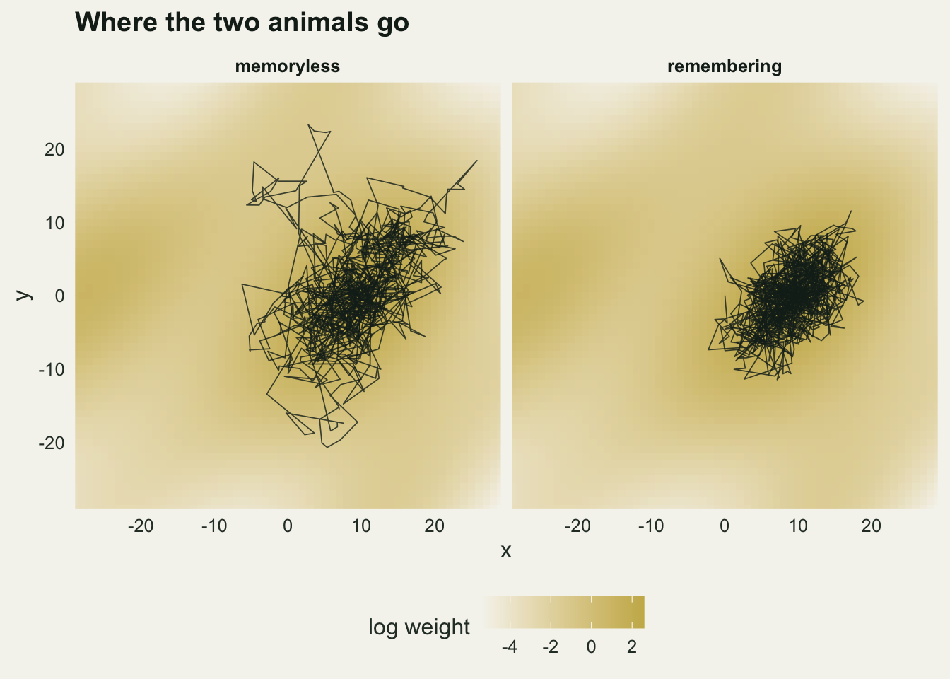

Figure 1: The first track of each animal over the full selection surface: both layers plus the pull towards home.

Averaged over the 48 tracks of each animal, the radius of gyration, the root mean squared distance of the fixes from their own centre, is 7.9 distance units for the memoryless animal and 4.8 for the remembering one. Both animals live on the same surface. Only one of them has a reason to come back to where it has been, beyond the surface itself.

Familiarity from past fixes only

The analysis follows the layout of the step selection posts on this site. Step t runs from fix P[t] to fix P[t + 1]; its ten available steps start at P[t] and draw their lengths from a gamma fitted by moments to the observed step lengths; and every model below carries step length and log step length next to its habitat terms, as integrated step selection analysis does. Steps 51 to 950 are analysed, so that every step has fixes both in its past set and in its future set.

The familiarity at the end of a used or available step is computed from P[1] to P[t - 50] only. The newest fix that counts is 50 positions older than the start of the step and 51 older than the used end, so neither end of the step, nor anything that happens after it, can enter. The placebo is the same kernel over P[t + 50] to the last fix of the track: places the animal has not reached yet, which no memory could use. Computing both for eleven end points at each of 900 steps is the expensive part of the post, so the chunk evaluates the kernel of every fix once per block of 50 steps and then sums only the fixes that qualify for each end point.

make_strata <- function(x, y) {
  tt <- (lag_fix + 1):(n_step - lag_fix)     # step t runs from P[t] to P[t + 1]
  sl <- sqrt(diff(x)^2 + diff(y)^2)
  shp <- mean(sl)^2 / var(sl)
  scl <- var(sl) / mean(sl)
  n_s <- length(tt)
  av_len <- matrix(rgamma(n_s * n_avail, shp, scale = scl), n_s)
  av_ang <- matrix(runif(n_s * n_avail, 0, 2 * pi), n_s)
  end_x <- cbind(x[tt + 1], x[tt] + av_len * cos(av_ang))
  end_y <- cbind(y[tt + 1], y[tt] + av_len * sin(av_ang))
  pts <- cbind(as.vector(end_x), as.vector(end_y))
  fix_xy <- cbind(x, y)
  n_fix <- length(x)
  t_pt <- rep(tt, n_avail + 1)
  m_past <- t_pt - lag_fix                   # P[1..t-lag]
  f_from <- t_pt + lag_fix                   # P[t+lag..n+1], the placebo
  s_past <- s_fut <- numeric(nrow(pts))
  q2 <- rowSums(fix_xy^2)
  for (blk in split(seq_len(nrow(pts)), (m_past - 1) %/% 50)) {
    arg <- 2 * tcrossprod(fix_xy, pts[blk, , drop = FALSE]) - q2
    arg <- sweep(arg, 2, rowSums(pts[blk, , drop = FALSE]^2))
    kern <- exp(pmin(arg, 0) / (2 * bw^2))   # n_fix x points, kernel of every fix
    lo <- min(m_past[blk]); hi <- max(m_past[blk])
    mid <- seq.int(lo + 1, length.out = hi - lo)
    s_past[blk] <- colSums(kern[seq_len(lo), , drop = FALSE]) +
      colSums(kern[mid, , drop = FALSE] * outer(mid, m_past[blk], "<="))
    f_lo <- min(f_from[blk]); f_hi <- max(f_from[blk])
    fmid <- seq.int(f_lo, length.out = f_hi - f_lo)
    s_fut[blk] <- colSums(kern[f_hi:n_fix, , drop = FALSE]) +
      colSums(kern[fmid, , drop = FALSE] * outer(fmid, f_from[blk], ">="))
  }
  n_fut <- n_fix - f_from + 1
  sl_m <- cbind(sl[tt], av_len)
  list(a = layer_a(end_x, end_y), b = layer_b(end_x, end_y), r2 = end_x^2 + end_y^2,
       sl = sl_m, lsl = log(sl_m),
       past = matrix(log(s_past / m_past + fam_eps), n_s),
       fut = matrix(log(s_fut / n_fut + fam_eps), n_s),
       x = end_x, y = end_y, t = tt)
}

set.seed(81003)
chk <- make_strata(trk_free$x[1, ], trk_free$y[1, ])
n_chk <- 200
i_chk <- sample(length(chk$x), n_chk)
t_chk <- rep(chk$t, n_avail + 1)[i_chk]
brute <- t(vapply(seq_len(n_chk), function(k) {
  p_idx <- seq_len(t_chk[k] - lag_fix)
  f_idx <- (t_chk[k] + lag_fix):(n_step + 1)
  kf <- function(idx) log(mean(exp(-((chk$x[i_chk[k]] - trk_free$x[1, idx])^2 +
                                     (chk$y[i_chk[k]] - trk_free$y[1, idx])^2) / (2 * bw^2))) + fam_eps)
  c(past = kf(p_idx), fut = kf(f_idx), newest = max(p_idx), oldest_fut = min(f_idx),
    used = t_chk[k] + 1)
}, numeric(5)))
fam_gap <- max(abs(c(brute[, "past"] - chk$past[i_chk], brute[, "fut"] - chk$fut[i_chk])))
stopifnot(fam_gap < 1e-8, all(brute[, "used"] - brute[, "newest"] == lag_fix + 1),
          all(brute[, "oldest_fut"] - brute[, "used"] == lag_fix - 1))

fit_ssf <- function(xl, iter = 60) {
  n_par <- length(xl)
  n_s <- nrow(xl[[1]])
  n_c <- ncol(xl[[1]])
  xm <- matrix(vapply(xl, as.vector, numeric(n_s * n_c)), ncol = n_par)
  sid <- rep(seq_len(n_s), n_c)
  used <- rep(c(TRUE, rep(FALSE, n_c - 1)), each = n_s)
  row_max <- function(m) m[cbind(seq_len(n_s), max.col(m, "first"))]
  probs <- function(b) {
    eta <- matrix(xm %*% b, n_s)
    pr <- exp(eta - row_max(eta))
    list(eta = eta, pr = as.vector(pr / rowSums(pr)))
  }
  loglik <- function(b) {
    eta <- matrix(xm %*% b, n_s)
    mx <- row_max(eta)
    sum(eta[, 1] - mx - log(rowSums(exp(eta - mx))))
  }
  centred <- function(pv) xm - rowsum(xm * pv, sid, reorder = TRUE)[sid, , drop = FALSE]
  b <- rep(0, n_par)
  ll <- loglik(b)
  for (it in seq_len(iter)) {
    pv <- probs(b)$pr
    xc <- centred(pv)
    step <- solve(crossprod(xc * sqrt(pv)), colSums(xc[used, , drop = FALSE]))
    fac <- 1
    repeat {
      b_new <- b + fac * step
      ll_new <- loglik(b_new)
      if (ll_new >= ll - 1e-9 || fac < 1e-4) break
      fac <- fac / 2
    }
    done <- abs(ll_new - ll) < 1e-10
    b <- b_new
    ll <- ll_new
    if (done) break
  }
  stopifnot(done)
  pv <- probs(b)$pr
  xc <- centred(pv)
  se <- sqrt(diag(solve(crossprod(xc * sqrt(pv)))))
  cbind(b = setNames(b, names(xl)), se = se)
}

own <- fit_ssf(chk[c("a", "past", "sl", "lsl")])
chk_long <- data.frame(stratum = rep(seq_len(nrow(chk$a)), n_avail + 1),
                       case = rep(c(1, rep(0, n_avail)), each = nrow(chk$a)),
                       a = c(chk$a), past = c(chk$past), sl = c(chk$sl), lsl = c(chk$lsl))
pkg <- summary(clogit(case ~ a + past + sl + lsl + strata(stratum), data = chk_long))$coefficients
fit_gap <- max(abs(own[, "b"] - pkg[, "coef"]), abs(own[, "se"] - pkg[, "se(coef)"]))
stopifnot(fit_gap < 1e-6)

On 200 end points drawn at random from one track, the block computation and a direct one written from the definition agree to within floating-point rounding for both covariates, and the stopifnot() line confirms for each of them that the newest fix in the past set is 51 positions before the used end and the oldest fix in the future set 49 positions after it. The hand-written fitter, a Newton-Raphson maximiser of the conditional likelihood used because two animals times 48 tracks times eight models would be too many calls to clogit() for a page that knits in a few minutes, agrees with clogit() from survival on every coefficient and standard error to \(7.5 \times 10^{-11}\).

Leave out a layer and the range, and memory appears

Every track of both animals is fitted with the same eight models. Each has layer A, step length and log step length, and then:

• past familiarity alone, with layer B and the home range left out;
• future familiarity alone, the placebo, with the same two left out;
• past and future familiarity together, with the same two left out;
• layer B, the squared distance from home and past familiarity, the full model;
• layer B, the squared distance from home and future familiarity;
• the squared distance from home and past familiarity, with only layer B left out;
• layer B and past familiarity, with only the home range left out;
• a polynomial surface in the coordinates and past familiarity, with layer B and the home range replaced by the surface.

A track calls memory when its familiarity coefficient is positive with a Wald z above 1.96, the two-sided five per cent test.

poly_surface <- function(st, degree = 6) {
  # every monomial u^i v^j with 0 < i + j <= degree, in standardised coordinates
  u <- (st$x - mean(st$x)) / sd(as.vector(st$x))
  v <- (st$y - mean(st$y)) / sd(as.vector(st$y))
  out <- list()
  for (i in 0:degree) for (j in 0:(degree - i)) {
    if (i + j > 0) out[[sprintf("u%dv%d", i, j)]] <- u^i * v^j
  }
  out
}
fit_track <- function(st) {
  mv <- st[c("sl", "lsl")]
  g <- function(vars, extra = NULL) {
    f <- fit_ssf(c(st[vars], mv, extra))
    z <- f[, "b"] / f[, "se"]
    c(b_past = if ("past" %in% vars) f["past", "b"] else NA,
      z_past = if ("past" %in% vars) z[["past"]] else NA,
      b_fut = if ("fut" %in% vars) f["fut", "b"] else NA,
      z_fut = if ("fut" %in% vars) z[["fut"]] else NA)
  }
  rbind(omit_past  = g(c("a", "past")),
        omit_fut   = g(c("a", "fut")),
        omit_joint = g(c("a", "past", "fut")),
        full_past  = g(c("a", "b", "r2", "past")),
        full_fut   = g(c("a", "b", "r2", "fut")),
        nob_past   = g(c("a", "r2", "past")),
        nor2_past  = g(c("a", "b", "past")),
        surf_past  = g(c("a", "past"), poly_surface(st)))
}
run_animal <- function(trk, seed) {
  set.seed(seed)
  lapply(seq_len(n_trk), function(i) fit_track(make_strata(trk$x[i, ], trk$y[i, ])))
}
res_free <- run_animal(trk_free, 81004)
res_mem <- run_animal(trk_mem, 81005)

collect <- function(res, animal) {
  arr <- simplify2array(res)             # model x statistic x track
  data.frame(animal = animal, model = rep(dimnames(arr)[[1]], dim(arr)[3]),
             track = rep(seq_len(dim(arr)[3]), each = dim(arr)[1]),
             b_past = as.vector(arr[, "b_past", ]), z_past = as.vector(arr[, "z_past", ]),
             b_fut = as.vector(arr[, "b_fut", ]), z_fut = as.vector(arr[, "z_fut", ]))
}
all_fits <- rbind(collect(res_free, "memoryless"), collect(res_mem, "remembering"))
z_crit <- qnorm(0.975)
summ <- function(animal, model, what = "past") {
  d <- all_fits[all_fits$animal == animal & all_fits$model == model, ]
  b <- d[[paste0("b_", what)]]
  z <- d[[paste0("z_", what)]]
  call <- mean(z > z_crit)
  c(mean = mean(b), se = sd(b) / sqrt(length(b)), call = call,
    call_se = sqrt(call * (1 - call) / length(b)), neg = mean(z < -z_crit))
}
s_ <- function(a, m, w = "past") summ(a, m, w)
om_free <- s_("memoryless", "omit_past")
om_mem <- s_("remembering", "omit_past")

With layer B and the home range left out, the memoryless animal’s familiarity coefficient averages 0.326 (Monte Carlo standard error 0.017), and 97.9 per cent of its tracks call memory (standard error 2.1 points). The animal has no memory at all. The remembering animal, fitted the same way, averages 0.862, larger than its true 0.5 because the term is carrying its memory and the missing structure together, and calls memory in 100 per cent of its tracks.

A reader of either fit would see a large, positive, highly significant coefficient on familiarity. Nothing on the page separates the memoryless animal from the remembering one except the size of the coefficient, and the size means nothing without a known scale for how much memory an animal ought to have.

row_lab <- c(omit_past = "B and range left out:\npast fixes",
             omit_fut = "B and range left out:\nfuture fixes (placebo)",
             full_past = "full model:\npast fixes",
             full_fut = "full model:\nfuture fixes (placebo)",
             surf_past = "surface instead of B and range:\npast fixes")
coef_df <- all_fits[all_fits$model %in% names(row_lab), ]
coef_df$b <- ifelse(grepl("fut", coef_df$model), coef_df$b_fut, coef_df$b_past)
coef_df$row <- factor(row_lab[coef_df$model], rev(row_lab))
set.seed(7)
coef_df$y_pos <- as.integer(coef_df$row) + ifelse(coef_df$animal == "remembering", 0.15, -0.15) +
  runif(nrow(coef_df), -0.08, 0.08)
ggplot(coef_df, aes(b, y_pos, colour = animal)) +
  geom_vline(xintercept = c(0, gam_mem), linetype = "dashed", colour = te_body, linewidth = 0.4) +
  geom_point(size = 1.3, alpha = 0.7) +
  scale_y_continuous(breaks = seq_along(levels(coef_df$row)), labels = levels(coef_df$row)) +
  scale_colour_manual(values = c(memoryless = te_rust, remembering = te_forest), name = NULL) +
  labs(x = "familiarity coefficient", y = NULL,
       title = "A familiarity coefficient without memory",
       subtitle = "dashed lines: no memory, and the remembering animal's 0.5") +
  theme_datasheet() +
  theme(legend.position = "bottom", plot.title.position = "plot")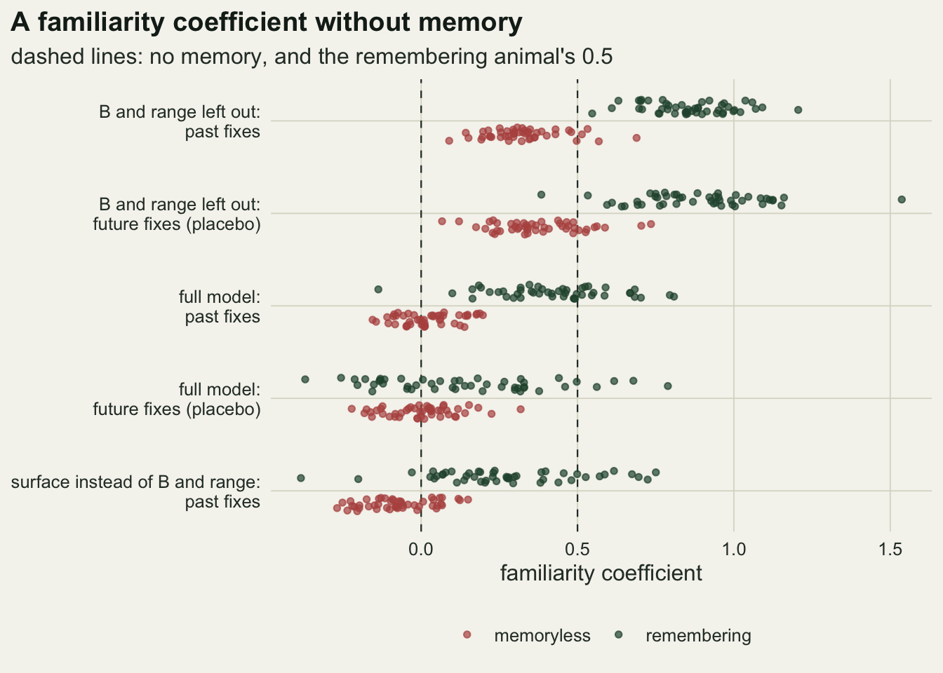

Figure 2: Familiarity coefficients, one point per track and model, for the memoryless and the remembering animal.

The future-fix placebo scores both animals alike

The placebo rests on a simple argument. If the past term measures memory, a term built the same way from fixes the animal has not made yet should do worse, because nothing can remember the future. If the future term does as well as the past one, the past term is picking up something other than memory.

pl_free <- s_("memoryless", "omit_fut", "fut")
pl_mem <- s_("remembering", "omit_fut", "fut")
pair_diff <- function(a) {
  d <- all_fits[all_fits$animal == a, ]
  b_p <- d$b_past[d$model == "omit_past"]
  b_f <- d$b_fut[d$model == "omit_fut"]
  c(diff = mean(b_f - b_p), se = sd(b_f - b_p) / sqrt(length(b_p)), ge = mean(b_f >= b_p))
}
pd_free <- pair_diff("memoryless")
pd_mem <- pair_diff("remembering")
side_by_side <- do.call(rbind, lapply(c("memoryless", "remembering"), function(a) {
  p_s <- s_(a, "omit_past")
  f_s <- s_(a, "omit_fut", "fut")
  data.frame(animal = a, past_mean = p_s[["mean"]], past_call = p_s[["call"]],
             future_mean = f_s[["mean"]], future_call = f_s[["call"]],
             call_se_max = max(p_s[["call_se"]], f_s[["call_se"]]))
}))
print(format(side_by_side, digits = 3), row.names = FALSE)

      animal past_mean past_call future_mean future_call call_se_max
  memoryless     0.326     0.979       0.374       0.938      0.0349
 remembering     0.862     1.000       0.885       1.000      0.0000

The printed table sets the two animals side by side, both fitted with layer B and the home range left out; the call columns are shares of tracks, and the last column is the larger of their two Monte Carlo standard errors. That is a plug-in standard error, which is zero when a share is exactly 0 or 1, as both are for the remembering animal; it does not mean the share is known exactly. For the memoryless animal the future term averages 0.374 and calls memory in 93.8 per cent of tracks. Track by track it is +0.047 above the past term on average (standard error 0.022), and it matches or beats the past term in 69 per cent of tracks. So far the placebo does its job: it says the past term is no better than a term that cannot be memory.

It says the same about the remembering animal. There the future term averages 0.885 and calls memory in 100 per cent of tracks; it differs from the past term by +0.023 on average (standard error 0.031) and matches or beats it in 56 per cent of tracks. An animal that returns to places it knows goes on returning to them, so its future fixes pile up where its past ones did, and the future layer inherits the memory signal along with the missing structure. Read side by side, the placebo gives the same verdict for an animal with no memory and for an animal whose memory is real. It is not a test of memory.

Past against future in one model

A sharper version puts both terms in one model, so that the past term is judged only on what it adds beyond the future one. This at least has the right logic: for a remembering animal, only the past fixes can explain the choices.

jt_free <- s_("memoryless", "omit_joint")
jt_free_fc <- s_("memoryless", "omit_joint", "fut")[["call"]]
jt_mem <- s_("remembering", "omit_joint")
jt_free_f <- s_("memoryless", "omit_joint", "fut")
jt_mem_f <- s_("remembering", "omit_joint", "fut")

With layer B and the home range still left out, the past term of the joint model averages 0.626 for the remembering animal and calls memory in 93.8 per cent of tracks, while its future term drops to 0.360. For the memoryless animal the past term averages 0.221 and the future term 0.250. Neither absorbs the other: the two layers behave like two noisy maps of the same missing structure, and each keeps a share of it. The past term therefore still calls memory in 60.4 per cent of tracks, with a Monte Carlo standard error of 7.1 points (the future term, for comparison, in 56.2 per cent). The contrast separates the two animals on average and fails for single tracks: an analyst with one memoryless animal would be told it remembers 60 times in a hundred.

jt <- all_fits[all_fits$model == "omit_joint", ]
ggplot(jt, aes(z_fut, z_past, colour = animal)) +
  geom_hline(yintercept = z_crit, linetype = "dashed", colour = te_body, linewidth = 0.4) +
  geom_vline(xintercept = z_crit, linetype = "dashed", colour = te_body, linewidth = 0.4) +
  geom_point(size = 2, alpha = 0.8) +
  scale_colour_manual(values = c(memoryless = te_rust, remembering = te_forest), name = NULL) +
  labs(x = "z of future familiarity", y = "z of past familiarity",
       title = "Past given future: a partial check",
       subtitle = "layer B and range left out; dashed lines: z = 1.96") +
  theme_datasheet() + theme(legend.position = "bottom")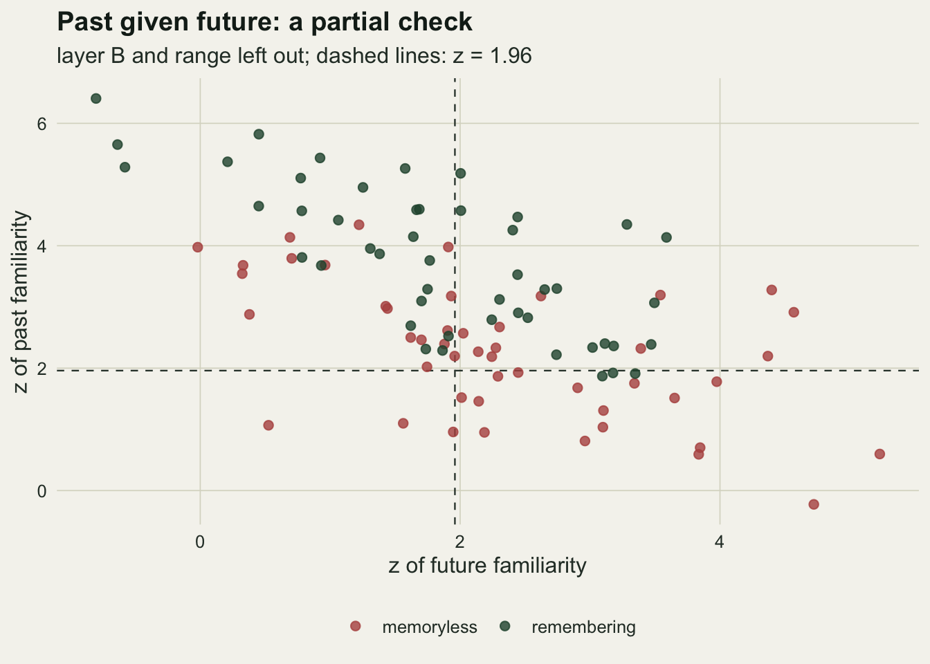

Figure 3: Wald z of the past and the future familiarity terms fitted together, with layer B and the range left out.

Putting the missing structure back

The full model contains layer B and the squared distance from home, the two pieces of structure the familiarity term was standing in for.

fl_free <- s_("memoryless", "full_past")
fl_mem <- s_("remembering", "full_past")
flf_free <- s_("memoryless", "full_fut", "fut")
flf_mem <- s_("remembering", "full_fut", "fut")
nob_free <- s_("memoryless", "nob_past")
nor2_free <- s_("memoryless", "nor2_past")
nob_mem <- s_("remembering", "nob_past")
nor2_mem <- s_("remembering", "nor2_past")

In the full model the memoryless animal’s familiarity coefficient averages 0.021 (standard error 0.013) and calls memory in 0.0 per cent of tracks (0 of 48; with none seen, the one-sided 95 per cent upper bound on the rate is 6.1 per cent); its future term calls memory in 2.1 per cent. The artefact is gone. The remembering animal keeps a coefficient of 0.422 (standard error 0.027), and its memory is detected in 68.8 per cent of tracks, with a standard error of 6.7 points. In the full model the comparison of past and future terms finally reads the right way for both animals. For the remembering animal the future term averages 0.137 against 0.422 for the past term, and calls memory in 8.3 per cent of tracks against 68.8; for the memoryless animal both terms sit near zero, the future one at 0.002. What removed the artefact was the specification, not the placebo; the placebo only became readable once the specification was right.

Both omissions contribute. With only layer B left out, the memoryless animal calls memory in 52.1 per cent of tracks; with only the home range left out, in 43.8 per cent; with both left out, in 97.9 per cent. The corresponding mean coefficients are 0.222, 0.157 and 0.326. For the remembering animal each single omission inflates the coefficient too, to 0.704 and 0.657.

The remembering animal’s coefficient in the full model falls short of its true 0.5, and that deserves a check before it is blamed on the available steps. The simulator kept the 30 candidates the animal actually chose from at every step, so the exact likelihood of the generating process can be fitted: a conditional logit on the true choice set, with nothing approximated. The same candidate covariates can also be given fresh choices drawn from the true weights, which cuts the link between the familiarity values and the choices that built them.

used_first <- function(m, pick) {
  ord <- t(vapply(pick, function(p) c(p, seq_len(n_cand)[-p]), integer(n_cand)))
  matrix(m[cbind(rep(seq_len(nrow(m)), n_cand), as.vector(ord))], nrow(m))
}
cs_fit <- vapply(seq_len(n_trk), function(i) {
  xl <- lapply(trk_mem$cand[c("a", "b", "r2", "fam")],
               function(arr) used_first(arr[i, , ], trk_mem$cand$pick[i, ]))
  fit_ssf(xl)[c("fam", "a", "b"), "b"]
}, numeric(3))
cs_mean <- rowMeans(cs_fit)
cs_se <- apply(cs_fit, 1, sd) / sqrt(n_trk)

set.seed(81006)
redraw_fit <- vapply(seq_len(n_trk), function(i) {
  covs <- lapply(trk_mem$cand[c("a", "b", "r2", "fam")], function(arr) arr[i, , ])
  w_log <- covs$a + covs$b - pull * covs$r2 + gam_mem * covs$fam
  new_pick <- max.col(w_log - log(-log(matrix(runif(length(w_log)), nrow(w_log)))), "first")
  fit_ssf(lapply(covs, used_first, pick = new_pick))[c("fam", "a", "b"), "b"]
}, numeric(3))
rd_mean <- rowMeans(redraw_fit)
rd_se <- apply(redraw_fit, 1, sd) / sqrt(n_trk)
pair_gap <- cs_fit[1, ] - redraw_fit[1, ]
pair_fr <- c(diff = mean(pair_gap), se = sd(pair_gap) / sqrt(n_trk))

On the animal’s own choices the exact likelihood returns a familiarity coefficient of 0.415 (standard error 0.024), almost exactly what the step selection fit returned, and layer A comes out at 1.278 (0.066) against a true 1. With fresh choices on the same candidates the familiarity, layer A and layer B coefficients are 0.470 (0.023), 1.069 (0.063) and 1.034 (0.038), each within 1.3 standard errors of its true value of 0.5, 1 or 1. So the shortfall does not come from the available steps. Taken alone, this comparison cannot say where it does come from: track by track, fresh choices give a familiarity coefficient 0.055 higher than the animal’s own choices (standard error 0.033), a gap of 1.7 standard errors. Track length says more. The chunk below refits the exact likelihood to the first 150, 300 and 450 analysed steps of every track, which is what a shorter track would give, because nothing in these fits looks forward, and pairs each length with fresh choices.

fam_only <- function(i, keep, pick) {
  xl <- lapply(trk_mem$cand[c("a", "b", "r2", "fam")], function(arr) used_first(arr[i, keep, ], pick))
  fit_ssf(xl)["fam", "b"]
}
fresh_pick <- function(i, keep) {
  covs <- lapply(trk_mem$cand[c("a", "b", "r2", "fam")], function(arr) arr[i, keep, ])
  w_log <- covs$a + covs$b - pull * covs$r2 + gam_mem * covs$fam
  max.col(w_log - log(-log(matrix(runif(length(w_log)), nrow(w_log)))), "first")
}
within_r2 <- function(i, keep) {
  # share of the within-step variation of familiarity that layer A, layer B and r2 reproduce
  cen <- function(m) as.vector(m - rowMeans(m))
  fam_c <- cen(trk_mem$cand$fam[i, keep, ])
  stat_c <- sapply(trk_mem$cand[c("a", "b", "r2")], function(arr) cen(arr[i, keep, ]))
  1 - sum(lm.fit(stat_c, fam_c)$residuals^2) / sum(fam_c^2)
}
n_an <- ncol(trk_mem$cand$pick)
len_ends <- c(150, 300, 450, n_an)
stopifnot(abs(fam_only(1, seq_len(n_an), trk_mem$cand$pick[1, ]) - cs_fit[1, 1]) < 1e-10)
set.seed(81007)
own_len <- fresh_len <- r2_len <- matrix(NA, n_trk, length(len_ends))
for (k in seq_along(len_ends)) {
  keep <- seq_len(len_ends[k])
  for (i in seq_len(n_trk)) {
    r2_len[i, k] <- within_r2(i, keep)
    if (len_ends[k] < n_an) {
      own_len[i, k] <- fam_only(i, keep, trk_mem$cand$pick[i, keep])
      fresh_len[i, k] <- fam_only(i, keep, fresh_pick(i, keep))
    }
  }
}
own_len[, length(len_ends)] <- cs_fit[1, ]      # the full length is the fit above
fresh_len[, length(len_ends)] <- redraw_fit[1, ]
mc_se <- function(m) apply(m, 2, sd) / sqrt(n_trk)
len_tab <- data.frame(steps = len_ends, own = colMeans(own_len), own_se = mc_se(own_len),
                      fresh = colMeans(fresh_len), fresh_se = mc_se(fresh_len),
                      overlap_r2 = colMeans(r2_len))
print(format(len_tab, digits = 3), row.names = FALSE)

 steps   own own_se fresh fresh_se overlap_r2
   150 0.504 0.0343 0.507   0.0350      0.668
   300 0.465 0.0289 0.489   0.0289      0.750
   450 0.435 0.0256 0.521   0.0281      0.794
   900 0.415 0.0239 0.470   0.0233      0.856

fall <- own_len[, 1] - own_len[, length(len_ends)]
fall_s <- c(mean = mean(fall), se = sd(fall) / sqrt(n_trk))

The table gives, at each length, the mean familiarity coefficient over the 48 tracks with its Monte Carlo standard error, first for the animal’s own choices and then for fresh ones, and in the last column the mean share of the variation of familiarity among the 30 candidates of a step that layer A, layer B and the squared distance from home reproduce together (a within-step R squared). On the animal’s own choices the coefficient falls from 0.504 at 150 steps to 0.415 at 900, a fall that averages 0.089 within tracks (standard error 0.024). With fresh choices it stays between 0.470 and 0.521, within 1.3 standard errors of 0.5 at every length. The shortfall is not a small-sample bias that a longer track removes: within these 900 steps it grows as the track lengthens. Over the same lengths the within-step R squared rises from 0.67 to 0.86: the longer the animal keeps returning, the more its familiarity map looks like the layers and the home range it selects. Fresh choices keep that overlap and cut the feedback from the choices to the covariate, and they show no clear shortfall; the animal’s own choices over the first 150 steps keep the feedback with less overlap, and show none either. In these fits the shortfall appears where the two come together, and every real track has both.

This whole section works because the omitted structure is known by construction. The chunk that simulates the animals defines layer B and the pull towards home, and the full model contains exactly those terms. A field analysis never has that luxury: the layer the animal selects and the analyst lacks is, by definition, not in the data.

dec_lab <- c(omit_past = "layer B\nand range", nob_past = "layer B\nonly",
             nor2_past = "range\nonly", full_past = "nothing",
             surf_past = "both, with\na surface")
dec <- do.call(rbind, lapply(c("memoryless", "remembering"), function(a)
  do.call(rbind, lapply(names(dec_lab), function(m) {
    s <- s_(a, m)
    data.frame(animal = a, left_out = dec_lab[[m]], call = s[["call"]], se = s[["call_se"]])
  }))))
dec$left_out <- factor(dec$left_out, dec_lab)
ggplot(dec, aes(left_out, call, colour = animal)) +
  geom_hline(yintercept = 0.05, linetype = "dashed", colour = te_body, linewidth = 0.4) +
  geom_errorbar(aes(ymin = pmax(call - 2 * se, 0), ymax = pmin(call + 2 * se, 1)),
                width = 0.15, linewidth = 0.5, position = position_dodge(width = 0.4)) +
  geom_point(size = 2.6, position = position_dodge(width = 0.4)) +
  scale_colour_manual(values = c(memoryless = te_rust, remembering = te_forest), name = NULL) +
  scale_y_continuous(limits = c(0, 1)) +
  labs(x = "left out of the model", y = "share of tracks calling memory",
       title = "What the familiarity term stands in for",
       subtitle = "dashed line: five per cent") +
  theme_datasheet() + theme(legend.position = "bottom")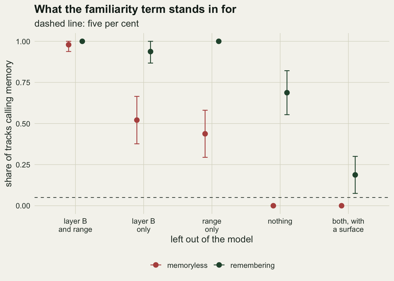

Figure 4: Share of tracks in which the past familiarity term is positive and significant at five per cent, by what the model leaves out. Bars are two Monte Carlo standard errors; a share of exactly 0 or 1 has a plug-in standard error of zero and so no bar.

A flexible surface is not the missing layer

When the missing structure has no name, the natural move, and the one the Hawkes post makes in time, is to give the model a flexible background. In space that means a smooth surface in the coordinates: here every monomial in the standardised coordinates up to degree 6, 27 terms, fitted in place of layer B and the home range. A static surface can in principle absorb any static preference, whatever its source, while a remembering animal’s familiarity changes as the track grows.

sf_free <- s_("memoryless", "surf_past")
sf_mem <- s_("remembering", "surf_past")
surf_shift <- function(a) {
  d <- all_fits[all_fits$animal == a, ]
  shift <- d$b_past[d$model == "surf_past"] - d$b_past[d$model == "full_past"]
  c(mean = mean(shift), se = sd(shift) / sqrt(length(shift)))
}
sh_free <- surf_shift("memoryless")
sh_mem <- surf_shift("remembering")
sh_gap_se <- sqrt(sh_free[["se"]]^2 + sh_mem[["se"]]^2)
n_terms <- length(poly_surface(chk))
stopifnot(n_terms == 27)

With the surface, the memoryless animal’s familiarity coefficient averages -0.073 (standard error 0.015); it calls memory in 0.0 per cent of tracks (again 0 of 48) and is significantly negative in 4.2 per cent. The false memory is gone, and the surface overshoots: the mean lies 4.7 standard errors below zero. The remembering animal pays for it. Its coefficient falls to 0.272 (standard error 0.034), 36 per cent below its value in the full model, and its memory is detected in 18.8 per cent of tracks, against 68.8 per cent in the full model. Much of that fall is the same downward push the surface gives the memoryless animal. Track by track, the surface moves the memoryless animal’s coefficient by -0.094 (standard error 0.009) and the remembering animal’s by -0.150 (standard error 0.025). The extra fall of the remembering animal, 0.056 with a standard error of 0.027, is only 2.1 standard errors, too little on 48 tracks to say that the surface also takes over memory itself, although a remembering animal’s space use, shaped by its memory as the tighter tracks above show, gives a static surface room to do so. Either way, a surface flexible enough to stand in for an unknown layer costs most of the power to detect the memory it was meant to reveal. The Hawkes post reports a related cost in time: part of the true excitation moved into its flexible background.

What to report

A familiarity or revisitation covariate is a function of the track, and the track records every reason the animal had to be where it was. Before a coefficient on it is read as memory, report how it changes as static structure is added: the habitat layers available, a term for the home range, and anything else that makes some places consistently attractive. In the simulations above the coefficient of a memoryless animal fell from 0.326 to 0.021 when the two missing pieces went in. The remembering animal’s coefficient shrank too, from 0.862 to 0.422, so a coefficient that shrinks as layers are added tells the reader what the term was carrying, not that there is no memory underneath.

Do not present a future-fix placebo as a test of memory. It flags the artefact in a memoryless animal and flags a genuinely remembering animal in the same way, so a placebo that scores as high as the past term says nothing about which animal is on the collar. If the placebo is reported at all, report it from the fullest model, where the past and future terms did separate for the remembering animal here, and say that the separation depended on the specification being right.

The joint past and future model is worth reporting as a partial check, with its limitation stated: in this simulation it called memory in 60 per cent of memoryless tracks. A population-level claim that rests on the share of animals with a significant past term inherits that rate.

Report the kernel bandwidth, the lag below which fixes do not count as familiar, and the floor inside the logarithm. Each changes what the covariate can absorb, and none of them was varied here.

If a flexible spatial surface is used to soak up unknown structure, say what it costs. Here it removed the false memory and cut the detection of real memory from 69 to 19 per cent of tracks. A memory coefficient that survives a flexible surface is stronger evidence than one that does not, but one that does not survive it is not evidence of no memory.

Honest limits

Everything here comes from one landscape: two sine-wave layers, a quadratic pull towards a single home, a gamma movement kernel with no directional persistence, 1000 steps per track and 30 candidates per step. The size of the artefact depends on how strongly the animal selects the missing layer, how tight its home range is and how long the track runs, and none of those was varied.

The full model removes the artefact because it contains exactly the terms the simulator used. That is the best case, and it is not available in the field. A partly right layer, or a home range term of the wrong shape, would leave part of the artefact in place; how much was not measured.

The home range here is a fixed pull towards a point, independent of memory. Van Moorter and colleagues (2009) showed that a home range can itself emerge from memory, in which case a home range term is not a nuisance to be controlled but a consequence of the process under study, and adding it could absorb real memory, a risk the polynomial surface here also carries.

Only one flexible surface was tried: a degree 6 polynomial with 27 terms. A smoother or rougher surface, splines or a spatial random field would trade the false memory against the real one at a different point. The conclusion that the trade exists is general; where it falls is specific to this surface.

The familiarity kernel, its bandwidth of 3, its lag of 50 steps and its floor are those of the pilot. The covariate fitted here is also exactly the rule the remembering animal used, which is a best case of its own: an analyst has to guess the bandwidth and the lag, and how much detection a wrong guess costs was not measured. Memory in real animals decays, weights recent visits, and may attach to particular resources rather than to places. A memory covariate built another way, for example from time since the last visit, could separate the animals better or worse than the one used here.

Each track is analysed alone. A population estimate built from many tracks would carry the same bias on average, and a count of significant tracks would carry the false-call rates above.

The shortfall of the remembering animal’s coefficient in the full model was examined only with the exact likelihood on the stored choice sets, at four track lengths inside the same simulated tracks. Within those 900 analysed steps it grew with track length. Longer tracks were not simulated, so whether it keeps growing or levels off is not known.

References

Oliveira-Santos LGR, Forester JD, Piovezan U, Tomas WM, Fernandez FAS 2016 Journal of Animal Ecology 85(2):516-524 (10.1111/1365-2656.12485)

Fagan WF, Lewis MA, Auger-Methe M, Avgar T, Benhamou S, Breed G, LaDage L, Schlagel UE, Tang WW, Papastamatiou YP, Forester J, Mueller T 2013 Ecology Letters 16(10):1316-1329 (10.1111/ele.12165)

Van Moorter B, Visscher D, Benhamou S, Borger L, Boyce MS, Gaillard JM 2009 Oikos 118(5):641-652 (10.1111/j.1600-0706.2008.17003.x)

Fortin D, Beyer HL, Boyce MS, Smith DW, Duchesne T, Mao JS 2005 Ecology 86(5):1320-1330 (10.1890/04-0953)

Avgar T, Potts JR, Lewis MA, Boyce MS 2016 Methods in Ecology and Evolution 7(5):619-630 (10.1111/2041-210X.12528)

Related tutorials

• Self-exciting events and the Hawkes process
• Integrated step selection analysis in R
• Validating a step selection model
• Step selection functions for animal movement